Coupled Oscillator: Coupled Mass-Spring System with Damping

Problem Statement

For the below system set up a set of state variable equations, and then solve. Assume all motion takes place in the vertical directions.

Fig. 1

Solution

Initial Values

For the upper mass:

$m_{1}=2kg{\frac {}{}}$

$k_{1}=10{\frac {N}{m}}$

$b_{1}=0.1{\frac {}{}}$

And for the lower mass:

$m_{2}=4kg{\frac {}{}}$

$k_{2}=12{\frac {N}{m}}$

$b_{2}=0.2{\frac {}{}}$

Initial Condition

We can have an input force, however, we are just going to have mass 2 pulled down 2 meters. Or in another words x_2 = 2 meters for our initial condition.

Find the Force Equations

First we need to sum forces in the y-direction for each block.

For mass 1:

$+\uparrow \sum F_{y_{1}}=m_{1}{\ddot {x}}_{1}\Rightarrow \ m_{1}{\ddot {x}}_{1}=-k_{1}x_{1}-2b_{1}{\dot {x}}_{1}+k_{2}(x_{2}-x_{1})+2b_{2}({\dot {x}}_{2}-{\dot {x}}_{1})$

For mass 2:

$+\uparrow \sum F_{y_{2}}=m_{2}{\ddot {x}}_{2}\Rightarrow \ m_{2}{\ddot {x}}_{2}=-k_{2}(x_{2}-x_{1})-2b_{2}({\dot {x}}_{2}-{\dot {x}}_{1})$

So if we put the equations above into the correct form we have:

${\ddot {x}}_{1}=-({\frac {k_{1}}{m_{1}}}+{\frac {k_{2}}{m_{1}}})x_{1}-({\frac {2b_{1}}{m_{1}}}+{\frac {2b_{2}}{m_{1}}}){\dot {x}}_{1}+{\frac {k_{2}}{m_{1}}}x_{2}+{\frac {2b_{1}}{m_{1}}}{\dot {x}}_{2}$

and

${\ddot {x}}_{2}={\frac {k_{2}}{m_{2}}}x_{1}+{\frac {2b_{2}}{m_{2}}}{\dot {x}}_{1}-{\frac {k_{2}}{m_{2}}}x_{2}-{\frac {2b_{2}}{m_{2}}}{\dot {x}}_{2}$

Note: Many people include the original length of the springs in the above equations, however if we take our initial reference point to be where the mass is in equilibrium, we do not need to include the initial spring length or gravity as an imput.

State Space Equation

The general form for the state equation is as shown below:

${\underline {\dot {x}}}={\widehat {A}}\,{\underline {x}}+{\widehat {B}}\,{\underline {u}}$

Where ${\widehat {M}}$ denotes a matrix and ${\underline {v}}$ denotes a vector.

If we let $x_{1}{\frac {}{}}$, ${\dot {x}}_{1}{\frac {}{}}$, $x_{2}{\frac {}{}}$, and ${\dot {x_{2}}}{\frac {}{}}$ be the state variables, then

${\begin{bmatrix}{\dot {x}}_{1}\\{\ddot {x}}_{1}\\{\dot {x}}_{2}\\{\ddot {x}}_{2}\end{bmatrix}}={\begin{bmatrix}0&1&0&0\\-({\frac {k_{1}}{m_{1}}}+{\frac {k_{2}}{m_{1}}})&-({\frac {2b_{1}}{m_{1}}}+{\frac {2b_{2}}{m_{1}}})&{\frac {k_{2}}{m_{1}}}&{\frac {2b_{1}}{m_{1}}}\\0&0&0&1\\{\frac {k_{2}}{m_{2}}}&{\frac {2b_{2}}{m_{2}}}&-{\frac {k_{2}}{m_{2}}}&-{\frac {2b_{2}}{m_{2}}}\\\end{bmatrix}}{\begin{bmatrix}x_{1}\\{\dot {x}}_{1}\\x_{2}\\{\dot {x}}_{2}\end{bmatrix}}+{\begin{bmatrix}0\\0\\0\\0\\\end{bmatrix}}{\begin{bmatrix}u\\\end{bmatrix}}$

Now we need to set up our output. The below is the general form of the output.

$y={\widehat {C}}\,{\underline {x}}+{\widehat {D}}\,{\underline {u}}$

If we want to output both positions and velocities of both masses we will use:

$y={\begin{bmatrix}1&0&0&0\\0&1&0&0\\0&0&1&0\\0&0&0&1\\\end{bmatrix}}{\begin{bmatrix}x_{1}\\{\dot {x}}_{1}\\x_{2}\\{\dot {x}}_{2}\end{bmatrix}}+{\begin{bmatrix}0\\0\\0\\0\end{bmatrix}}{\begin{bmatrix}u\\\end{bmatrix}}$

Eigenvalues

If we solve the A matrix for the eigenvalues using Matlab we get:

$\lambda _{1}=-0.1729+3.5780i\,$

$\lambda _{2}=-0.1729-3.5780i\,$

$\lambda _{3}=-0.0271+1.0808i\,$

$\lambda _{4}=-0.0271-1.0808i\,$

Eigenvectors

Now that we have our eigenvalues, we can use them to find the eigenvectors. Again using Matlab we get:

$k_{1}={\begin{bmatrix}0.0124+0.2568i\\-0.9211\\-0.0015-0.0786i\\0.2814+0.0084i\end{bmatrix}}$

$k_{2}={\begin{bmatrix}0.0124-0.2568i\\-0.9211\\-0.0015+0.0786i\\0.2814-0.0084i\end{bmatrix}}$

$k_{3}={\begin{bmatrix}-0.0121-0.3535i\\0.3824-0.0034i\\-0.0145-0.5794i\\0.6266\end{bmatrix}}$

$k_{4}={\begin{bmatrix}-0.0121+0.3535i\\0.3824+0.0034i\\-0.0145-0.5794i\\0.6266\end{bmatrix}}$

Diagonalized A Matrix

With the above eigenvectors we also get the diagonalized A matrix which we will denote as D:

${\mathbf {D}}={\begin{bmatrix}-0.1729+3.5780i&0&0&0\\0&-0.1729-3.5780i&0&0\\0&0&-0.0271+1.0808i&0\\0&0&0&-0.0271-1.0808i\end{bmatrix}}$

Solving

We know that the T inverse matrix is just made up from the eigenvector columns, so:

${\mathbf {T^{-1}}}={\begin{bmatrix}0.0124+0.2568i&0.0124-0.2568i&-0.0121-0.3535i&-0.0121+0.3535i\\-0.9211&-0.9211&0.3824-0.0034i&0.3824+0.0034i\\-0.0015-0.0786i&-0.0015+0.0786i&-0.0145-0.5794i&-0.0145+0.5794i\\0.2814+0.0084i&0.2814-0.0084i&0.6266&0.6266\end{bmatrix}}$

It then follows that the T matix is:

${\mathbf {T}}={\begin{bmatrix}-0.0070-1.6408i&-0.4576-0.0222i&0.0070+1.0012i&0.2793+0.0050i\\-0.0070+1.6408i&-0.4576+0.0222i&0.0070-1.0012i&0.2793-0.0050i\\-0.0188+0.2221i&0.2052+0.0070i&0.0103+0.7274i&0.6726+0.0169i\\-0.0188-0.2221i&0.2052-0.0070i&0.0103-0.7274i&0.6726-0.0169i\end{bmatrix}}$

Now we can use the equation for a transfer function to help us solve through the use of matrix exponentials.

${\bar {z}}={\mathbf {T}}{\bar {x}}\,$

This can be rearranged by multiplying T-inverse to the left side of the equations.

${\mathbf {T^{-1}}}{\bar {z}}={\bar {x}}\,$

Now we can bring in the standard form of a state space equation

${\dot {\bar {x}}}={\mathbf {A}}{\bar {x}}$

Combining the two equations we then get

${\mathbf {T^{-1}}}{\dot {\bar {z}}}={\mathbf {AT^{-1}}}{\bar {z}}$

Multiplying both sides of the equation on the left by T we get

${\dot {\bar {z}}}={\mathbf {TAT^{-1}}}{\bar {z}}$

${\dot {\bar {z}}}={\mathbf {\hat {A}}}{\bar {z}}$

where

${\mathbf {D}}={\mathbf {TAT^{-1}}}$

If we take the Laplace transform of the above D matrix from the previous secton and use the below equation:

${\bar {z}}=e^{{\mathbf {D}}t}{\bar {z}}(0)$

where

$e^{{\mathbf {D}}t}={\begin{bmatrix}e^{(-0.1729+3.5780i)t}&0&0&0\\0&e^{(-0.1729-3.5780i)t}&0&0\\0&0&e^{(-0.0271+1.0808i)t}&0\\0&0&0&e^{(-0.0271-1.0808i)t}\end{bmatrix}}$

We then substitute this equation back into

${\bar {x}}={\mathbf {T^{-1}}}{\bar {z}}$

and get

${\bar {x}}={\mathbf {T^{-1}}}e^{{\mathbf {D}}t}{\bar {z}}(0)$

${\bar {x}}={\mathbf {T^{-1}}}e^{{\mathbf {D}}t}{\mathbf {T}}{\bar {x}}(0)$

Notice here that

$e^{{\mathbf {A}}t}={\mathbf {T^{-1}}}e^{{\mathbf {D}}t}{\mathbf {T}}$

Which gives us

${\begin{bmatrix}0.0124+0.2568i&0.0124-0.2568i&-0.0121-0.3535i&-0.0121+0.3535i\\-0.9211&-0.9211&0.3824-0.0034i&0.3824+0.0034i\\-0.0015-0.0786i&-0.0015+0.0786i&-0.0145-0.5794i&-0.0145+0.5794i\\0.2814+0.0084i&0.2814-0.0084i&0.6266&0.6266\end{bmatrix}}$

${\begin{bmatrix}e^{(-0.1729+3.5780i)t}&0&0&0\\0&e^{(-0.1729-3.5780i)t}&0&0\\0&0&e^{(-0.0271+1.0808i)t}&0\\0&0&0&e^{(-0.0271-1.0808i)t}\end{bmatrix}}$

${\begin{bmatrix}-0.0070-1.6408i&-0.4576-0.0222i&0.0070+1.0012i&0.2793+0.0050i\\-0.0070+1.6408i&-0.4576+0.0222i&0.0070-1.0012i&0.2793-0.0050i\\-0.0188+0.2221i&0.2052+0.0070i&0.0103+0.7274i&0.6726+0.0169i\\-0.0188-0.2221i&0.2052-0.0070i&0.0103-0.7274i&0.6726-0.0169i\end{bmatrix}}$

Note: All of the above matrices are supposed to be multiplied in the horizontal, but they are put in the vertical to save space so that you don't need to scroll over.

As in Johnathan Schreven's problem, the solution to the above matrix multiplication is huge, therefore I am not going to include it here. It does however work out.

Graphical Representation

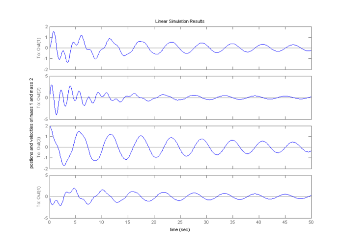
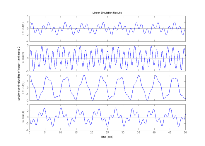
Since the solution above is so long below is a graphical representation of the solution. I could not figure out how to change the y-axis labels on each of the four graphs per one solution. So the first two are position and velocity of mass 1 and the second two are position and velocity of mass two. Positions are in meters and velocities are in meters per second. Figure one is with the initial value of damping, and figure 2 is the same system with no damping.

Fig. 1

Fig. 2

As we can see, there is a huge difference between the two graphs. This shows us that even if damping is small, there can be a huge difference in the output.

The matlab code used is shown below:

Tstop = 50; % Total time run
npts = 500; % Number of points per second
mag = 0;    % This has to do with input exp. (0 = nothing, 1 = step)
m1=2;       % Mass, Spring constants, and Damping coefficients
m2=4;
k1=10;
k2=12;
b1= .1;
b2= .2;
A=[       0                 1             0           0
   -(k1/m1+k2/m1)  -(2*b1/m1+2*b2/m1)  (k2/m1)    (2*b1/m1)
          0                 0             0           1
      ( k2/m2)          (2*b2/m2)     -(k2/m2)   -(2*b2/m2)];
B=[0 0 0 0]';              % A, B, C, D are the matrices from our equations
C=[1 0 0 0
   0 1 0 0
   0 0 1 0
   0 0 0 1];
D=[0
   0
   0
   0];
X0=[0 0 2 0]';             % The initial value matrix
sys1 = ss(A,B,C,D);        % Setting up the system for the state equations
t= linspace(0,Tstop,npts); % Setting up the time axis
u= mag*ones(size(t));      % The input
lsim(sys1,u,t,X0);         % lsim is the solver for the state equations
xlabel('time');
ylabel('postions and velocities of mass 1 and mass 2');

Again, the only difference between the graphs are the damping coefficients.

---

Written by: David Steinweg