Using the DFT
Jump to navigation
Jump to search
This is what we get when we sample the signal at 3Hz
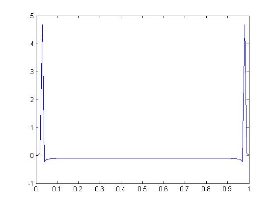
Taking the original signal and applying the DFT we get this graph:
Now taking the DFT of this sampled signal, we get a graph like this:
Script for matlab:
clear all;
t=0:.01:2;
T=1/3;
ts=0:T:2;
f1=2;
f2=1/0.125;
x = sin(2*pi*ts); %this is the function
plot(ts,sin(2*pi*ts),'r-',t,sin(2*pi*t)); % plot the original signal and the signal sampled at 3Hz
X = fft(x); % take the DFT
pause (2);
plot (ts,X); %plot the DFT of the signal sampled at 3Hz
pause (4);
x=sin(2*pi*t);
plot(t,x);
pause(2);
X = fft(x);
plot(t,X); %plot the DFT of the original signal

