FIR Filter Example Code for Octave

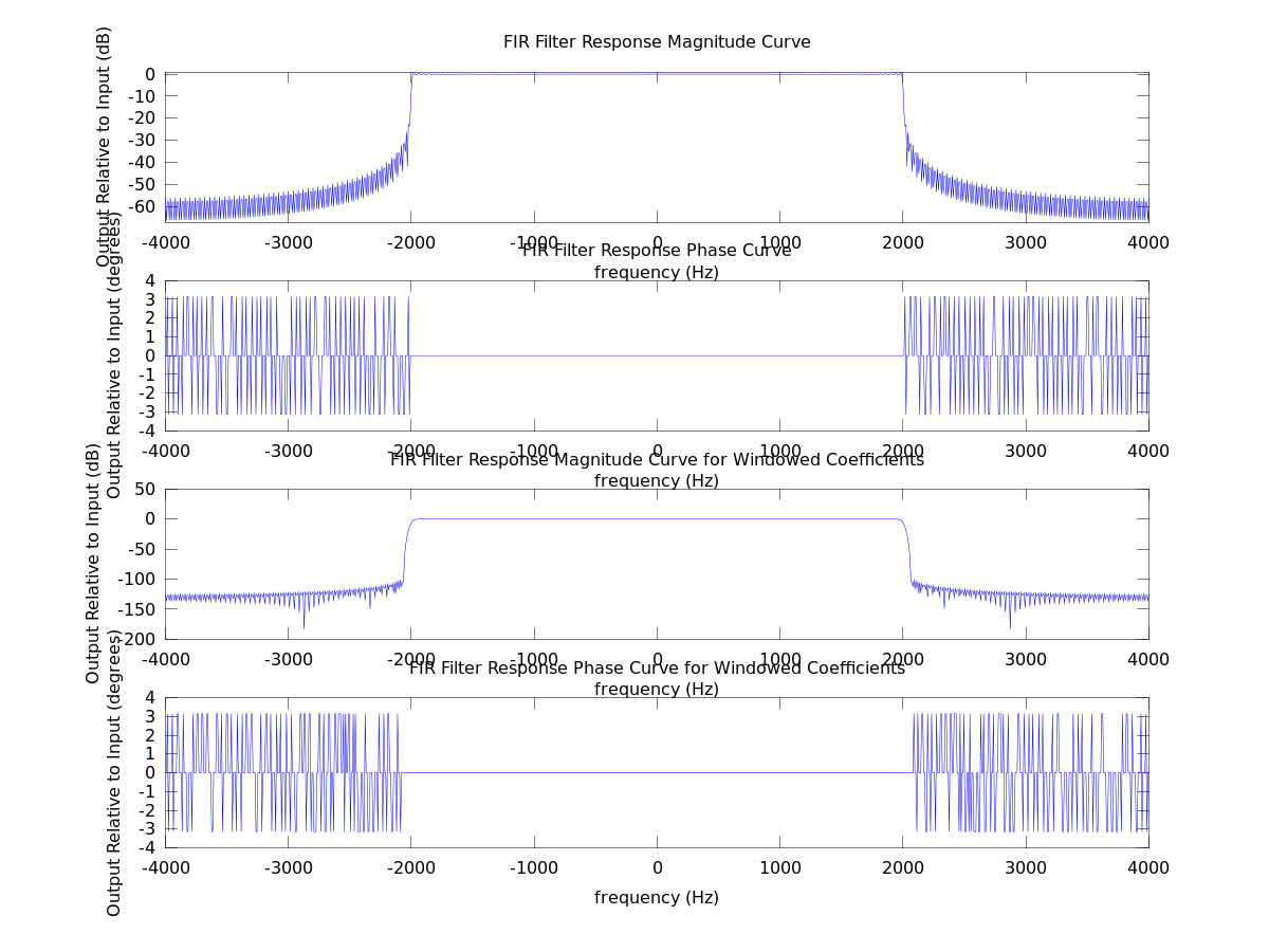
% This demonstration shows the magnitude and phase response for an FIR filter
% of 2M+1 elements whose ideal response is a low pass filter with cutoff
% frequency of fs/4.
% This also demonstrates the effect of using a window function like
% the Kaiser window to reduce the side lobes of the filter.
%
% Written by Rob Frohne.  Feel free to copy or use any way you wish!
clear;
M=200;
T=1/8000;
f=-1/2/T:1/1000/T:1/2/T;
sum = zeros(size(f));
h1=[];
clf;
w=kaiser(2*M+1,10);
for m=-M:-1;
    h=sin(pi*m/2)/pi/m;
    h1=[h1,h];
    sum = sum + h*exp(-i*2*pi*f*m*T);
end
sum = sum + .5;
h1=[h1,.5];
for m=1:M;
    h=sin(pi*m/2)/pi/m;
    h1=[h1,h];
    sum = sum + h*exp(-i*2*pi*f*m*T);
end   
hw=(w'.*h1);
sumw=zeros(size(f));
for m=-M:M;
    sumw=sumw + hw(m+M+1).*exp(-i*2*pi*f*m*T);
end
figure(1);
subplot(4,1,1), plot(f,20*log10(abs(sum)));
title('FIR Filter Response Magnitude Curve');
ylabel('Output Relative to Input (dB)');
xlabel('frequency (Hz)');
subplot(4,1,2), plot(f,angle(sum));
title('FIR Filter Response Phase Curve');
xlabel('frequency (Hz)');
ylabel('Output Relative to Input (degrees)')
subplot(4,1,3), plot(f,20*log10(abs(sumw)));
title('FIR Filter Response Magnitude Curve for Windowed Coefficients');
ylabel('Output Relative to Input (dB)');
xlabel('frequency (Hz)');
subplot(4,1,4), plot(f,angle(sumw));
title('FIR Filter Response Phase Curve for Windowed Coefficients');
xlabel('frequency (Hz)');
ylabel('Output Relative to Input (degrees)')
%plot(20*log10(abs(fft(h1))))

% Try the filter out.
Totaltime = 2;
%speak('Make the signal!');
%[nt,Fs] = recordsound(Totaltime, 1/T, 1);
t = 0:T:5;
nt = sin(2*pi*(1/20/T.*t).*t);
Fs = 1/T;
%speak('Here is the unfiltered signal.');
soundsc(nt,Fs);
figure(2);
Y=filter(h1,1,nt);
Yw=filter(hw,1,nt);
%speak('Here is the filtered signal.');
soundsc(Y,Fs);
%speak('Here is the filtered signal with windowed coefficients.');
soundsc(Yw,Fs);
subplot(3,1,1), plot(nt);
title('Unfiltered Signal');
subplot(3,1,2), plot(Y);
title('Filtered Signal');

subplot(3,1,3), plot(Yw);
title('Filtered Signal');

The figure showing the frequency response is below. Running the file you will hear the results as well.