Fourier Series Example Script
Jump to navigation
Jump to search
Sampled Fourier Series
This is a script that plots a few terms of the Fourier series of a square wave and then plots some samples of it in red *'s. You can copy this and paste it into your editor and run it from octave or just paste it into an octave window to see the plot.
% This script plots a Fourier Series for a Square Wave
clf;
t=0:.01:10;
T=2.5
M=50
sum1=0;
for m=1:2:M,
    sum1 = sum1+4/m/pi*sin(m*pi/2)*cos(2*pi*m*t/T);
end
plot(t,sum1,'b-',t(1:10:end),sum1(1:10:end),'r*')
title('Fourier Series Representation of a Square Wave')
xlabel('time (seconds)')
ylabel('Function')
grid on;
axis([0,10,-2,2])
legend('Five Terms','Five Terms Sampled')
print("squarewave.png","-dpng")  % Prints the plot to a png file called squarewave.png
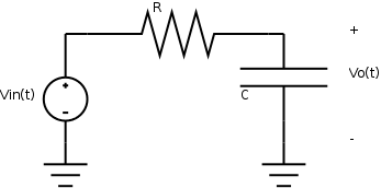
Fourier Series Solution for Sinusoidal Steady State Response of a Low Pass Filter
This goes with the class notes for October 1, 2010.
clf;
t=0:.01:10;
T=pi;
R=2;
C=1;
M=101;
vin=0;
current =0;
for n=1:2:M,
	vin = vin+1./(n.*pi).*(3.*sin(pi.*n./2)...
-sin(3.*n.*pi./2)).*cos(2.*pi.*n.*t./T);
	current = current+1./(sqrt(R.^2+1./...
((2.*pi.*n./T).^2*C.^2))).*1./(n.*pi).*(3.*sin(pi.*n./2)...
-sin(3.*n.*pi./2)).*cos(2.*pi.*n.*t./T-atan2(-1,2*pi*n/T*R*C));
end
vout=vin-R.*current;
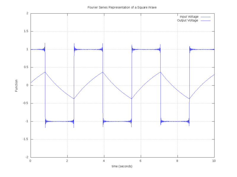
plot(t,vin,'b-',t,vout)
title('Fourier Series Representation of a Square Wave')
xlabel('time (seconds)')
ylabel('Function')
grid on;
axis([0,10,-2,2])
legend('Input Voltage','Output Voltage')
print("LowPass.png","-dpng")  % Prints the plot to a png file called squarewave.png
The output produces a nice plot.

