In Phase (I) and Quadrature (Q) Signals of Image Reject Mixers
In radios (and other electronics) it is often desired to shift a signal's frequency. This is the job of the mixer circuit. The mixer is represented by a circle with a multiply symbol inside it, as shown below. 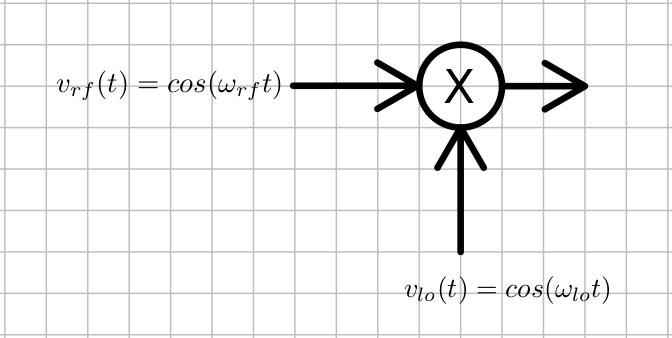
If we multiply $cos(\omega_{lo}t)$ with $cos(\omega_{rf}t)$ we get ${cos[\pm(\omega_{lo}-\omega_{rf})t] + cos[\pm(\omega_{lo}+\omega_{rf})t]}/2$. This contains the desired term, $cos[\pm(\omega_{lo}-\omega_{rf}]t]$, which does the frequency shift. The $\pm$ is because $cos(-x) = cos(x)$. Negative frequencies are indistinguishable from positive frequencies from the cosine's point of view. This brings up the question of what we mean by negative frequencies, but put that aside for now as we examine how a mixer would work in a software defined radio receiver. To be clear, both $\omega_{rf}$ and $\omega_{lo}$ are positive numbers (so, for example, $-\omega_{rf} < 0$) in this discussion.
The block diagram of a simple software defined receiver is shown below. 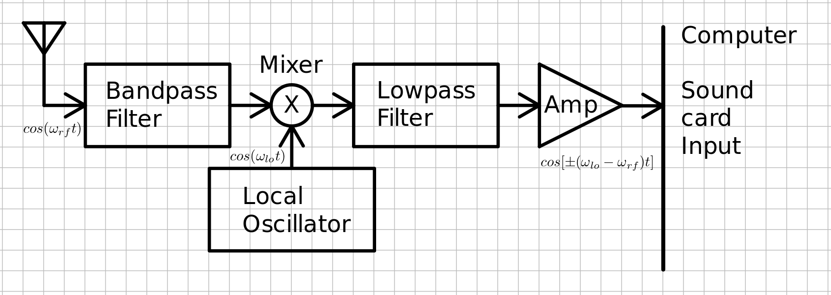
In order to tune in stations at their different frequencies, the frequency shift needs to be adjustable. Generally the frequency to be shifted is the frequency of an adjustable oscillator, called the local oscillator. The frequency of the local oscillator is $f_{lo} = \omega_{lo}/(2\pi)$ and is set by some type of control on the local oscillator. The low pass filter just after the mixer removes the $cos[\pm(\omega_{lo}+\omega_{rf})t]$ term from the signals impinging on the sound card, which converts these low frequencies to digital samples. There is still a problem though, because there are actually still two signals in $cos[\pm(\omega_{lo}-\omega_{rf}]t]$ that make it to the data stream from the sound card, one for the "+" and one for the "-" from the $\pm$. When we are listening to the receiver, we cannot tell if it was the "+" or the "-" term that caused what we are listening to, and sometimes two different radio stations will end up getting shifted right on top of one another, one from the "+" term and one from the "-" term. The "+" term and the "-" term are known as images of each other. It would be very nice if we could send enough data to the computer so it could distinguish between these two signals. This is actually twice as much data as we are sending with the simple SDR above. Fortunately sound cards often have stereo inputs.
To understand how to solve the image problem above, we need to understand what we mean by negative frequency, and get a more intuitive idea how we can tell the images apart. For a moment, consider a propeller, of unit length, spinning in the counterclockwise direction at 100 revolutions or cycles per second. See the figure below. 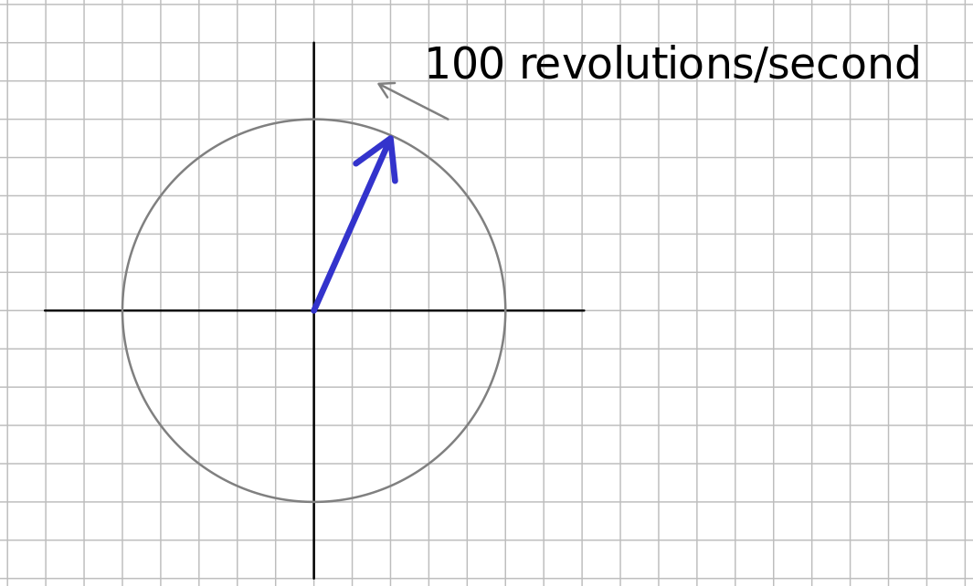
Let's call that a positive frequency of 100 Hz. What would a negative frequency of 100 Hz be? It seems obvious that it would be the propeller spinning the opposite direction (clockwise). If you look at the propeller from the bottom perspective you would see the tip going back and forth like a cosine wave in time. Looking only from the bottom, you could not tell if it was spinning clockwise or counterclockwise. However, if you could look from the bottom and from the right side ($90^{\circ}$ from the bottom), you could tell which way it was turning. Remember that the parametric equation describing the tip of the propeller spinning counterclockwise at frequency $\omega$ is $\vec v = cos(\omega t) \hat {\mathbf i} + sin(\omega t)\hat {\mathbf j}$. If you spin in the clockwise direction (change $\omega$ to $-\omega$), and the $sin(\omega t)\hat {\mathbf j}$ becomes $-sin(\omega t)\hat {\mathbf j}$, because $sin(-x) = -sin(x)$. Another way to represent this circular rotation is in the complex plane, where the real part of the number is in the $\hat{\mathbf i}$ direction and the imaginary number is in the $\hat{\mathbf j}$ direction. Euler's identity which says $e^{j\omega t} = cos(\omega t) + jsin(\omega t)$ shows that $e^{j\omega t}$ represents a counter clockwise spin of the propeller, and $e^{-j\omega t}$ represents a clockwise spin of the propeller. The animation below shows this.
import matplotlib.pyplot as plt
import matplotlib.animation
import matplotlib.ticker as plticker
import numpy as np
from IPython.display import HTML

t = np.linspace(0, 2)
x = np.cos(np.pi*t)
y = np.sin(np.pi*t)
fig, ax = plt.subplots(nrows=2, ncols=2,
                       gridspec_kw={'hspace': 0.3, 'wspace': 0.2}, figsize=(8, 8));
plt.close();
ax[0][0].set_aspect(1)
ax[0][0].axis([-1, 1, -1, 1])
ax[0][1].set_aspect(1)
ax[1][0].set_aspect(1)
ax[0][1].axis([0, 2, -1, 1])
ax[1][0].axis([-1, 1, 0, 2])
ax[1][1].axis('off')
x_title = '$\mathscr {Re}[e^{j\omega t}]$'
y_title = '$\mathscr {Im}[e^{j\omega t}]$'
x_label = '$\mathscr {Im}$'
y_label = '$\mathscr {Re}$'
t_label = 't (s)'
ax[0][0].set_xlabel(x_label)
ax[0][1].set_xlabel(t_label)
ax[1][0].set_xlabel(x_label)
ax[0][0].set_ylabel(y_label)
ax[0][0].xaxis.set_label_position("top")
ax[0][0].xaxis.tick_top()
ax[0][1].yaxis.set_label_position("right")
ax[0][1].yaxis.tick_right()
ax[1][0].yaxis.set_label_position("right")
ax[1][0].yaxis.tick_right()
axis_linewidth = 0.75
real_color = 'cyan'
im_color = 'magenta'
complex_color = 'green'
ax[0][0].axhline(0, color=real_color, linewidth=axis_linewidth)
ax[0][0].axvline(0, color=im_color, linewidth=axis_linewidth)
ax[0][1].axhline(0, color='black', linewidth=axis_linewidth)
ax[1][0].axvline(0, color='black', linewidth=axis_linewidth)
ax[0][0].set_title('$e^{j\omega t}$')
ax[0][1].set_title(y_title)
ax[1][0].set_title(x_title)
loc = plticker.MultipleLocator(base=1.0)
for i in range(len(ax)):
    for j in range(len(ax[0])):
        ax[i, j].xaxis.set_major_locator(loc)
        ax[j, i].yaxis.set_major_locator(loc)
l1, = ax[0][0].plot([], [], '.', color=complex_color)
l2, = ax[0][1].plot([], [], '.', color=im_color)
l3, = ax[1][0].plot([], [], '.', color=real_color)
ax[0][1].legend([l2],[y_title])
ax[1][0].legend([l3],[x_title])

def animate(i):
    l1.set_data(x[:i], y[:i])
    l2.set_data(t[:i], y[:i])
    l3.set_data(x[:i], t[:i])

ani = matplotlib.animation.FuncAnimation(fig, animate, frames=len(t), interval=200);

HTML(ani.to_html5_video())  # For just the animation, no controls.
#HTML(ani.to_jshtml())  # Animation with controls.
The phasor above has positive frequency and advances in the counterclockwise direction. The phasor below has negative frequency and advances in the clockwise direction. The difference between them is seen in the sign of the imaginary component. This is how you tell if the frequency is positive or negative.
t = np.linspace(0, 2)
x = np.cos(-np.pi*t)
y = np.sin(-np.pi*t)
fig, ax = plt.subplots(nrows=2, ncols=2,
                       gridspec_kw={'hspace': 0.3, 'wspace': 0.2}, figsize=(8, 8));
plt.close();
ax[0][0].set_aspect(1)
ax[0][0].axis([-1, 1, -1, 1])
ax[0][1].set_aspect(1)
ax[1][0].set_aspect(1)
ax[0][1].axis([0, 2, -1, 1])
ax[1][0].axis([-1, 1, 0, 2])
ax[1][1].axis('off')
x_title = '$\mathscr {Re}[e^{-j\omega t}]$'
y_title = '$\mathscr {Im}[e^{-j\omega t}]$'
x_label = '$\mathscr {Im}$'
y_label = '$\mathscr {Re}$'
t_label = 't (s)'
ax[0][0].set_xlabel(x_label)
ax[0][1].set_xlabel(t_label)
ax[1][0].set_xlabel(x_label)
ax[0][0].set_ylabel(y_label)
ax[0][0].xaxis.set_label_position("top")
ax[0][0].xaxis.tick_top()
ax[0][1].yaxis.set_label_position("right")
ax[0][1].yaxis.tick_right()
ax[1][0].yaxis.set_label_position("right")
ax[1][0].yaxis.tick_right()
axis_linewidth = 0.75
real_color = 'cyan'
im_color = 'magenta'
complex_color = 'green'
ax[0][0].axhline(0, color=real_color, linewidth=axis_linewidth)
ax[0][0].axvline(0, color=im_color, linewidth=axis_linewidth)
ax[0][1].axhline(0, color='black', linewidth=axis_linewidth)
ax[1][0].axvline(0, color='black', linewidth=axis_linewidth)
ax[0][0].set_title('$e^{-j\omega t}$')
ax[0][1].set_title(y_title)
ax[1][0].set_title(x_title)
loc = plticker.MultipleLocator(base=1.0)
for i in range(len(ax)):
    for j in range(len(ax[0])):
        ax[i, j].xaxis.set_major_locator(loc)
        ax[j, i].yaxis.set_major_locator(loc)
l1, = ax[0][0].plot([], [], '.', color=complex_color)
l2, = ax[0][1].plot([], [], '.', color=im_color)
l3, = ax[1][0].plot([], [], '.', color=real_color)
ax[0][1].legend([l2],[y_title])
ax[1][0].legend([l3],[x_title])

def animate(i):
    l1.set_data(x[:i], y[:i])
    l2.set_data(t[:i], y[:i])
    l3.set_data(x[:i], t[:i])

ani = matplotlib.animation.FuncAnimation(fig, animate, frames=len(t), interval=200);

HTML(ani.to_html5_video())  # For just the animation, no controls.
#HTML(ani.to_jshtml())  # Animation with controls.
Suppose we were to observe the wave from orthogonal perspectives as described above, and passed the data from those perspectives into the left and right channels respectively, then we could tell which way the vector was spinning, and so would have enough information to listen to only the signals spinning in one way or the other. The block diagram for this receiver is shown below. 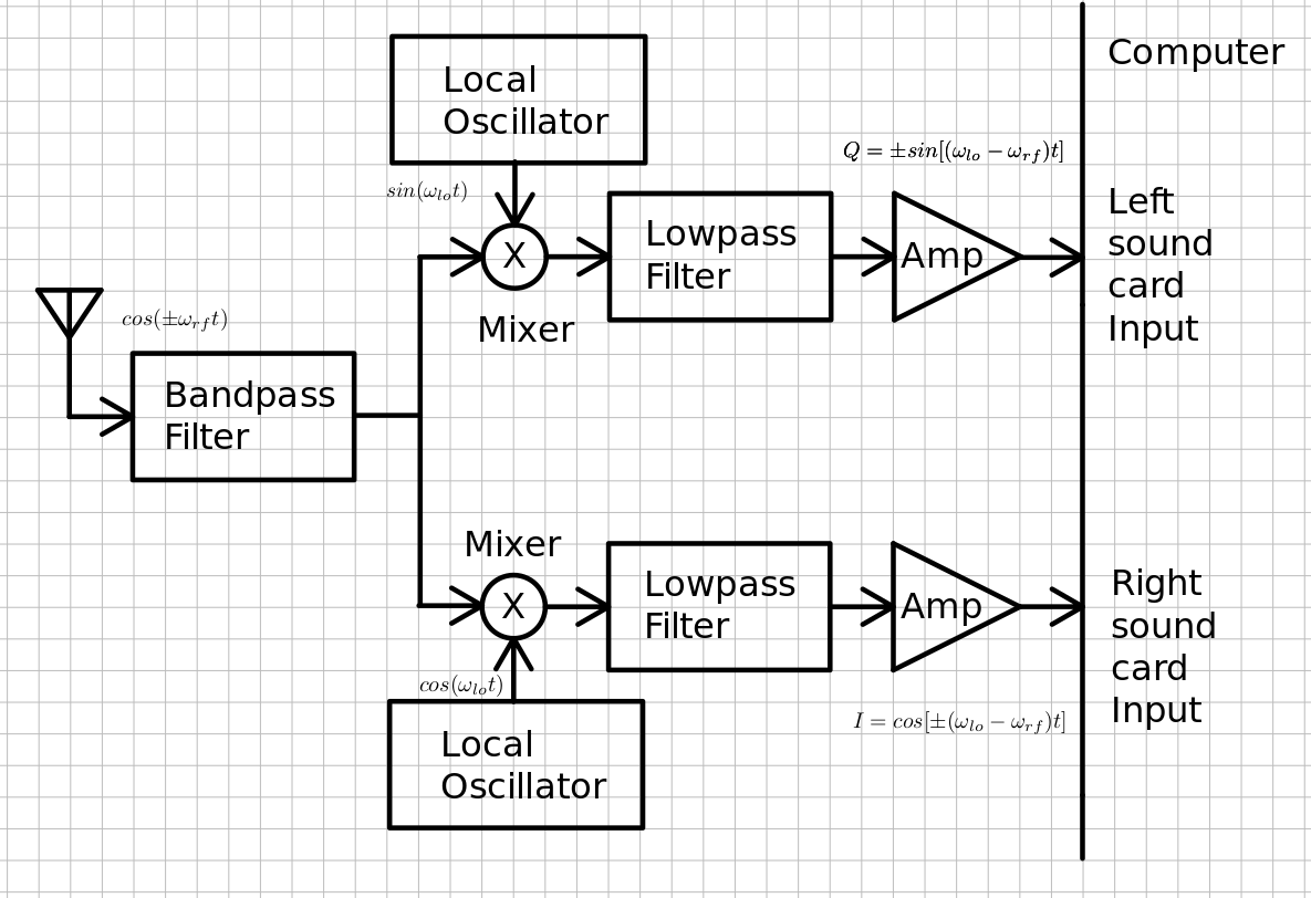
This mixer system for this is known as an image reject mixer, and the signal shifted by the $cos(\omega_{lo}t)$ is known as the in phase signal (I), and the signal shifted by $sin(\omega_{lo}t)$ (or in some receivers by $-sin(\omega_{lo}t)$) is known as the quadrature signal (Q).