Complex Numbers
An imaginary number, $j$ is defined by the property $j^2=-1$. A complex number has a real part, $a$ and an imaginary part, $jb$ where $a$ and $b$ are real numbers. The complex number, $a+jb$, may be viewed as a two dimensional vector of sorts, where the real part, $a$, is one component, and the imaginary part, $jb$ is viewed as the other component. There are two ways of representing complex numbers, polar and rectangular. This is based on a famous formula credited to Leonard Euler, $e^{j\theta} = cos\theta + jsin\theta$. Richard Feynman called this formula "our jewel" and "the most remarkable formula in mathematics." See the figure below.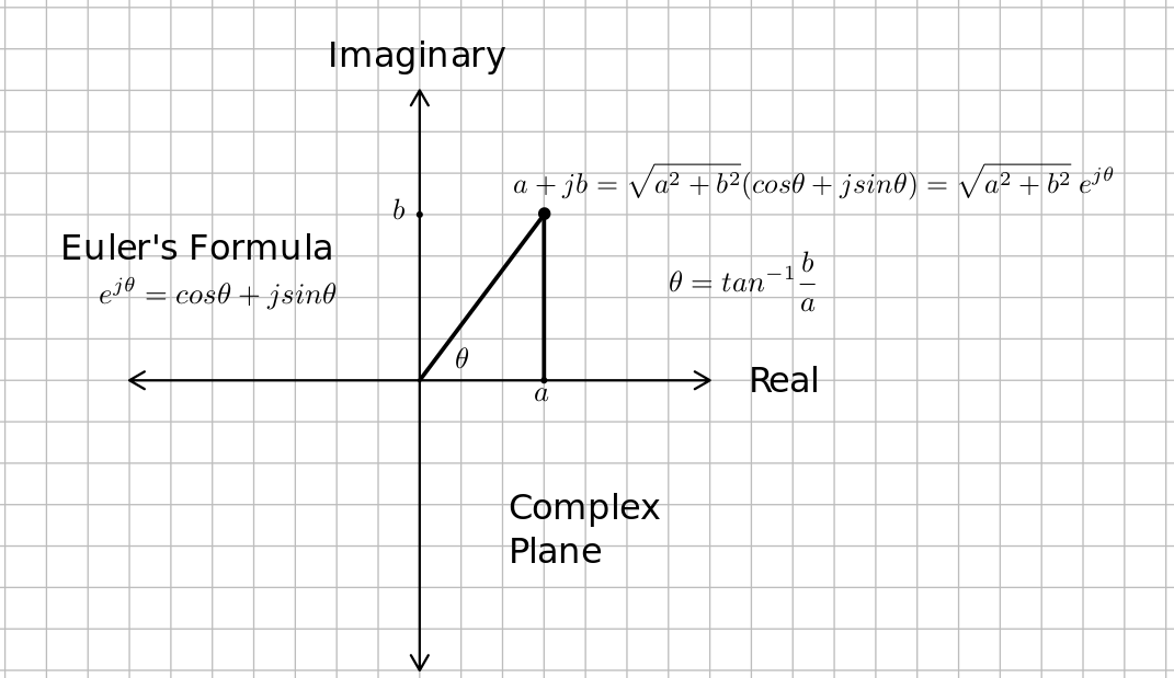
Multiplication by $j$ is rotation counterclockwise by $90^\circ$ or $\pi/2$. For example, $j = e^{j\pi/2}$ and $e^{j \pi} = -1$. The reciprocal of the imaginary number ($1/j$) is $-j$.
The complex conjugate of a complex number is written with a superscript $*$ so the complex conjugate of $a+jb$ is written $(a+jb)^*$ and is equal to $a-jb$. You can take the complex conjugate of any function by replacing every $j$ with a $-j$. The real part of a complex number is $ \mathscr {Re}(a+jb) = 1/2[(a+jb) + (a+jb)^*] = a$, or half the sum of the complex number and its complex conjugate. The imaginary part of a number is half the difference between the number and its complex conjugate. That is $\mathscr{Im}[u] = 1/2(u-u^*)$. When you wish to multiply, divide, or exponentiate a complex numbers, the polar form is easiest to use. When you wish to add or subtract complex numbers,the rectangular form is most convenient.
The magnitude of a complex number, $a+jb$ is the sum of the squares of its real and imaginary parts and is written with using magnitude bars, as with vectors. For example, the magnitude of a complex number $a+jb$ is written as $|a+jb| = \sqrt{a^2+b^2}$. You can write $|a+jb|^2 = (a+jb)(a-jb) = (a+jb)(a+jb)^*$. Note that the magnitude of any complex number is a positive real number and is the distance from the origin to that number. See the figure above.
The angle of a complex number, $a+jb$ is $tan^{-1}b/a$. You have to be very careful when using your calculator, because $tan^{-1}(\frac{-1}{1}) \ne tan^{-1}(\frac{1}{-1})$ and $tan^{-1} (\frac{-1}{-1}) \ne tan^{-1}(\frac{1}{1})$. They are $180^\circ$ apart. Some calculators have a rectangular to polar conversion function, and it requires you enter both $a$ and $b$. The atan2(y, x) can also be used in some programming languages and it takes the abmiguity from the arctangent function.
Phasors Application
In July 1893 Charles Steinmetz published the method of phasors which simplified solving sinusoidal steady state circuits problems. The key to this method was noticing that $e^{j\omega t}$ is the eigenfunction of differentiation in time, so that circuits driven by $e^{j\omega t}$ produce differential equations that turn into algebraic equations, and that solutions for circuits driven by sources of the form $V_m cos(\omega t + \phi)$ could be solved by applying $V_m e^{j(\omega t + \phi)}$ and then the real part of that solution would be the desired response for the original circuit.
A linear timeinvariant system is linear. Being linear means that a linear combination of inputs has the same linear combination of the outputs. Linearity can be broken down into two properties, proportionality (if you double the input, you double the output), and superposition (if input one produces output one, and input two produces output two, then if the input is the sum of inputs one and two, the output will be the sum of outputs one and two). See the table below.
| Input Signal into the System | Output Signal from the System | Reason for this Output |
|---|---|---|
| $x_1(t)$ | $y_1(t)$ | Given |
| $x_2(t)$ | $y_2(t)$ | Given |
| $\alpha x_1(t)$ | $\alpha y_1(t)$ | Proportionality |
| $x_1(t) + x_2(t)$ | $y_1(t) + y_2(t)$ | Superposition |
| $\alpha x_1(t)+\beta x_2(t)$ | $\alpha y_1(t)+\beta y_2(t)$ | Linearity |
Suppose we have a linear time invariant system, and the the impulse response is given as shown below.
| Input Signal into the System | Output Signal from the System | Reason for this Output |
|---|---|---|
| $\delta (t)$ | $h(t)$ | Given |
| $\delta (t-t_0)$ | $h(t-t_0)$ | Time invariance |
| $x(t_0) \delta (t-t_0)$ | $x(t_0)h(t-t_0)$ | Linearity |
| $x(t) =\int_{-\infty}^{\infty}x(t_0) \delta (t-t_0)dt_0$ | $\int_{-\infty}^{\infty}x(t_0)h(t-t_0) dt_0$ | Linearity |
| $e^{j2\pi f t}$ | $\int_{-\infty}^{\infty}e^{j2\pi ft_0}h(t-t_0) dt_0$ | The above line |
The last output integral can be simplified with a substitution of variables to: $$\int_{-\infty}^{\infty}e^{j2\pi ft_0}h(t-t_0) dt_0 = \int_{-\infty}^{\infty}e^{j2\pi f(t-t_0)}h(t_0) dt_0 =e^{j2\pi ft} \int_{-\infty}^{\infty}e^{-j2\pi fu}h(u) du = e^{j2\pi ft} H(f)$$ where $H(f)$ is the Fourier Transform of $h(t)$ and the phasor transfer function of the system. From this we see that $e^{j2\pi ft}$ is the eigenfunction of the system, and that the eigen value for that particular $f$ is $H(f)$.
Application to a Circuit
Suppose we wish to understand how the following circuit 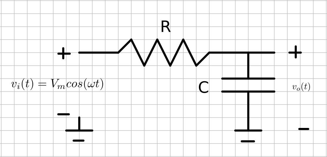 treats a sinusoidal source as the frequency is varied in steady state. Steady state means after transients have died down, so in the language of mathematics, we want the particular solution to the governing differential equation. In engineering we often call this the forced response. The radian frequency $\omega = 2\pi f$.
Using Kirchoff's current law, we can write the differential equation $$C \frac {dv_o}{dt} + \frac{v_o(t) - v_i(t)}{R} = 0$$ Suppose we used $v_i(t) = V_m e^{j\omega t} = V_m cos(\omega t) + jV_m sin(\omega t)$ as the excitation instead of $v_i(t) = V_m cos(\omega t)$. Using the ideas of linearity, every part of the solution due to $jsin(\omega t)$ will be imaginary. The solution we want is the part that is real, because it is due to the excitation, $V_m cos(\omega t)$. If you stare at the differential equation above with this $v_i(t)$, you will eventually decide a good guess for the solution would be something like $v_o(t) = \bar V e^{j\omega t}$ where $\bar V$ is a complex constant. Substituting this guess into the differential equation, $$ j\omega C \bar V e^{j\omega t}+ \frac {\bar Ve^{j\omega t} -V_me^{j\omega t}}{R} = 0$$ $$ j\omega C \bar V + \frac {\bar V -V_m}{R} = 0$$ $$ \bar V = \frac{V_m/(j\omega C)}{R+1/(j\omega C)} = \frac{V_m}{1+j\omega RC} = \frac{V_m}{\sqrt{1+\omega^2R^2C^2}}e^{-jtan^{-1}(\omega RC)}$$
Note that $H(f)$ from the table above is $H(f) = H(\omega/(2\pi)) = \bar V / V_m =\frac{1}{\sqrt{1+\omega^2R^2C^2}}e^{-jtan^{-1}(\omega RC)}$. This is known as the transfer function. The ouput is $H(\omega/(2\pi)) V_me^{j\omega t}$ as shown in the table above.
The output due to $v_i(t) = V_m cos(\omega t)$ is $$ v_o(t) = \mathscr {Re}[\bar V e^{j\omega t}] = \mathscr {Re}\left[\frac{1}{\sqrt{1+\omega^2R^2C^2}}e^{j(\omega t - tan^{-1}(\omega RC)}\right]= \frac{1}{\sqrt{1+\omega^2R^2C^2}}cos({\omega t-tan^{-1}(\omega RC)})$$ using Euler's formula.
Euler's formula was intimately involved in this example. Visualize the phasor rotating with radian frequency around the complex plane as seen in the demo below. Note that $cos(\omega t)$ is the projection on the real axis, and $sin(\omega t)$ is the projection on the imaginary axis.
import matplotlib.pyplot as plt
import matplotlib.animation
import matplotlib.ticker as plticker
import numpy as np
from IPython.display import HTML

t = np.linspace(0, 2)
x = np.cos(np.pi*t)
y = np.sin(np.pi*t)

fig, ax = plt.subplots(nrows=2, ncols=2,
                       gridspec_kw={'hspace': 0.3, 'wspace': 0.2}, figsize=(8, 8));
plt.close();
ax[0][0].set_aspect(1)
ax[0][0].axis([-1, 1, -1, 1])
ax[0][1].set_aspect(1)
ax[1][0].set_aspect(1)
ax[0][1].axis([0, 2, -1, 1])
ax[1][0].axis([-1, 1, 0, 2])
ax[1][1].axis('off')
x_title = '$\mathscr {Re}[e^{j\omega t}]$'
y_title = '$\mathscr {Im}[e^{j\omega t}]$'
x_label = '$\mathscr {Im}$'
y_label = '$\mathscr {Re}$'
t_label = 't (s)'
ax[0][0].set_xlabel(x_label)
ax[0][1].set_xlabel(t_label)
ax[1][0].set_xlabel(x_label)
ax[0][0].set_ylabel(y_label)
ax[0][0].xaxis.set_label_position("top")
ax[0][0].xaxis.tick_top()
ax[0][1].yaxis.set_label_position("right")
ax[0][1].yaxis.tick_right()
ax[1][0].yaxis.set_label_position("right")
ax[1][0].yaxis.tick_right()
axis_linewidth = 0.75
real_color = 'cyan'
im_color = 'magenta'
complex_color = 'green'
ax[0][0].axhline(0, color=real_color, linewidth=axis_linewidth)
ax[0][0].axvline(0, color=im_color, linewidth=axis_linewidth)
ax[0][1].axhline(0, color='black', linewidth=axis_linewidth)
ax[1][0].axvline(0, color='black', linewidth=axis_linewidth)
ax[0][0].set_title('$e^{j\omega t}$')
ax[0][1].set_title(y_title)
ax[1][0].set_title(x_title)
loc = plticker.MultipleLocator(base=1.0)
for i in range(len(ax)):
    for j in range(len(ax[0])):
        ax[i, j].xaxis.set_major_locator(loc)
        ax[j, i].yaxis.set_major_locator(loc)
l1, = ax[0][0].plot([], [], '.', color=complex_color)
l2, = ax[0][1].plot([], [], '.', color=im_color)
l3, = ax[1][0].plot([], [], '.', color=real_color)
ax[0][1].legend([l2],[y_title])
ax[1][0].legend([l3],[x_title])

def animate(i):
    l1.set_data(x[:i], y[:i])
    l2.set_data(t[:i], y[:i])
    l3.set_data(x[:i], t[:i])

ani = matplotlib.animation.FuncAnimation(fig, animate, frames=len(t), interval=200);

HTML(ani.to_html5_video())  # For just the animation, no controls.
#HTML(ani.to_jshtml())  # Animation with controls.
Euler's indentity is so important, because $e^{j2\pi ft}$ is the eigen function of every linear time invariant system, which means solving for outputs of this very important class of systems is most easily accomplished if excitations can be made with linear combinations of $e^{j2\pi ft}$. Essentially what was done in the example above is to write $$cos(\omega t) = \mathscr{Re}[e^{j\omega t}] = 1/2[e^{j\omega t} + (e^{j\omega t})^*] = 1/2[e^{j\omega t} + e^{-j\omega t}] $$
Fortunately Joseph Fourier discovered how to write most any function of $t$ as a linear combination of $e^{j2\pi ft}$ for different frequencies, $f$. He started with the periodic functions as described in the notebook, Complex Fourier Series. He then took the limit as the period gets very large, and obtained the Fourier Transform which works for non-periodic functions. This made Euler's formula and complex numbers even more important in science and engineering.