Designing Custom Frequency Responses for FIR Filters

Designing your own custom frequency response into the FIR filter is really very easy. All that needs to be modified are the coefficients for the FIR filter. Presented here are only the formulas to tailor the cutoff frequencies to your liking. If you have a little familiarity with the calculus, I invite you to investigate the references.

Three steps are involved in calculating filter coefficients. The first is to use the formulas
 
 

and
 

to find the un-windowed I and Q filter coefficients.  (The funny p above is supposed to be pi.)  The desired lower cutoff frequency is fL and the upper one is fH; fS is the sampling rate (8000 Hz in this case). M is the number of filter coefficients you use. The software is presently uses 256 coefficients for each channel. This is the reason m goes from -128 to 127. Note the similarity between the I and Q coefficients. The only change between them is the sine terms becoming cosine terms. This provides the 90 degrees of phase delay necessary. If you are modifying the response curve for AM or DSB, set hQ(m) = 0.

 The next step is to apply the windowing function. The purpose of the windowing function is to reduce the sidelobes (bumps in the filter response caused by Gibbs phenomenon). The Kaiser window I used is a semi-optimum window function that allows you to trade sidelobe levels for sharpness of the transition region, by varying the parameter ß. I used ß = 8.0. Other windowing functions are possible. To apply the window function, multiply each coefficient by its window value given by:

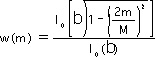
where I sub 0 is the zeroth-order modified Bessel Function of the first kind and b is supposed to be beta.

 The final step is to plot the response curve actually obtained (neglecting of course quantization and finite wordlength effects). If you like the response, great, if not go back to step one. Remember that the dynamic range of the codec limits the stopband attenuation to about 80 db. The equation for computing this frequency response is:

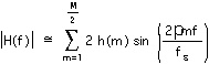
(The funny p above is supposed to be pi.)  The expression is exact for an odd number of coefficients, M, and very close for M even. (All these steps are automated if you have access to MATLAB. The MATLAB code uses an exact relation for any M, even or odd.) It will also plot the theoretical opposite sideband rejection if everything except the FIR filter is perfect. The software which does that is available on my web site, http://www.wwc.edu/~frohro/....