Laplace transforms:Series RLC circuit

Laplace Transform Example: Series RLC Circuit

Problem

Given a series RLC circuit with $R=10Ohms$, $L=0.1H$, and $C=10^{-5}F$, having power source $v(t)=10cos(20t)$, find an expression for $i(t)$ if $i(0)=0A$ and $v_{c}(0)=0V$.

Solution

We begin with the general formula for voltage drops around the circuit:

$v(t)=Ri+L{\dfrac {di}{dt}}+{\dfrac {1}{C}}\int {idt}$

Substituting numbers, we get

$10cos(20t)=10i+0.1{\dfrac {di}{dt}}+10^{5}\int {idt}$

$\Rightarrow cos(20t)=i+0.01{\dfrac {di}{dt}}+10000\int {idt}$

Now, we take the Laplace Transform and get

${\dfrac {s}{s^{2}+20^{2}}}=I+0.01[sI-i(0)]+10000{\dfrac {I}{s}}$

Using the fact that $i(0)=0A$, we get

${\dfrac {s}{s^{2}+400}}=I+0.01sI+10000{\dfrac {I}{s}}$

$\Rightarrow {\dfrac {s^{2}}{s^{2}+400}}=sI+0.01s^{2}I+10000I$

$\Rightarrow {\dfrac {s^{2}}{s^{2}+400}}=(0.01s^{2}+s+10000)I$

$\Rightarrow I(s)={\dfrac {s^{2}}{(s^{2}+400)(0.01s^{2}+s+10000)}}$

Using partial fraction decomposition, we find that

$I(s)={\dfrac {1.0004-4.003*10^{-8}s}{0.01s^{2}+s+10000}}+{\dfrac {4.003*10^{-6}s-0.04002}{s^{2}+400}}$

$\Rightarrow I(s)={\dfrac {100.04-4.003*10^{-6}s}{s^{2}+100s+1000000}}+{\dfrac {4.003*10^{-6}s-0.04002}{s^{2}+400}}$

$\Rightarrow I(s)={\dfrac {100.04-4.003*10^{-6}s}{(s+50)^{2}+997500}}+{\dfrac {4.003*10^{-6}s-0.04002}{s^{2}+400}}$

$\Rightarrow I(s)={\dfrac {100.038}{(s+50)^{2}+(50{\sqrt {399}})^{2}}}-{\dfrac {4.003*10^{-6}s+.002}{(s+50)^{2}+(50{\sqrt {399}})^{2}}}+{\dfrac {4.003*10^{-6}s}{s^{2}+20^{2}}}-{\dfrac {0.04002}{s^{2}+20^{2}}}$

$\Rightarrow I(s)={\dfrac {10.038}{50{\sqrt {399}}}}{\dfrac {50{\sqrt {399}}}{(s+50)^{2}+(50{\sqrt {399}})^{2}}}-4.003*10^{-6}{\dfrac {s+50}{(s+50)^{2}+(50{\sqrt {399}})^{2}}}+4.003*10^{-6}{\dfrac {s}{s^{2}+20^{2}}}-{\dfrac {0.04002}{20}}{\dfrac {20}{s^{2}+20^{2}}}$

Finally, we take the inverse Laplace transform to obtain

$i(t)=0.01e^{-50t}sin(998.8t)-(4.003*10^{-6})e^{-50t}cos(998.8t)+(4.003*10^{-6})cos(20t)-0.002sin(20t)\,$

which is our answer.

Initial/Final Value Theorems

We now want to use the Initial and Final Value Theorems on this problem.

The Initial Value Theorem states that

$\lim _{s\to \infty }sF(s)=f(0^{+})$

$\Rightarrow \lim _{s\to \infty }{\dfrac {s^{3}}{(s^{2}+400)(0.01s^{2}+s+10000)}}=i(0)$

$\Rightarrow i(0)=0$

In addition, when we actually evaluate $i(0)$ from our equation for $i(t)$, we find it to be 0 as well. So, things check out there.

The Final Value Theorem states that

$\lim _{s\to 0}sF(s)=f(\infty )$

$\Rightarrow \lim _{s\to 0}{\dfrac {s^{3}}{(s^{2}+400)(0.01s^{2}+s+10000)}}=i(\infty )$

$\Rightarrow i(\infty )=0$

This time, when we actually evaluate i(∞) from the equation for $i(t)$, we find it to be undefined. So here, the Final Value Theorem tells us something that is not necessarily true (in fact, because we have oscillating functions, we know that i(∞) will not be zero).

Bode Plot

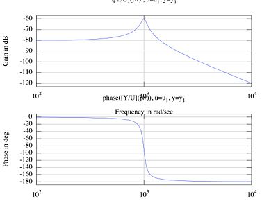
To get a Bode plot, we use the transfer function:

$H(s)={\dfrac {1}{0.01s^{2}+s+10000}}$

We then use a program such as Octave or MATLAB to obtain the Bode plot, which looks like this:

Bode Plot

Break Points

We can also use break points to approximate and/or validate the Bode plot.

The break points of our function are determined by the transfer function

$H(s)={\dfrac {1}{0.01s^{2}+s+10000}}={\dfrac {100}{(s^{2}+100s+1000000)}}$

The break points are:

$1000\downdownarrows$(40db/decade down)

Looking at the top part of the Bode plot, we see that the graph is indeed going down at roughly 40db/decade at 1000.

Convolution

We now want to show how convolution can achieve the same result as our Laplace Transform methods.

Convolution means that

$i(t)=v(t)*h(t)=\int _{0}^{t}{v(\tau )h(t-\tau )d\tau }$

where $h(t)$ is the inverse Laplace transform of the transfer function.

Here,

$h(t)=0.1e^{-2500t}sin(998.7t)\,$

Thus,

$i(t)=\int _{0}^{t}{10cos(20\tau )(.01e^{-2500(t-\tau )}sin(998.7(t-\tau ))d\tau }$

$\Rightarrow i(t)=-.000014e^{-2500t}cos(998.7t)-.000034e^{-2500t}sin(998.7t)+.000014cos(20t)+.0000002sin(20t)$

This doesn't look exactly like the answer we got above, but we expect this since convolution doesn't take initial conditions into account.

State Equations

To begin the demonstration of a new method (state space equations), we want to translate the system into a set of state equations:

${\begin{bmatrix}i\\{\dfrac {di}{dt}}\end{bmatrix}}={\begin{bmatrix}0&1\\1000000&10\end{bmatrix}}{\begin{bmatrix}\int {idt}\\i\end{bmatrix}}+{\begin{bmatrix}0\\100cos(20t)\end{bmatrix}}$

$i={\begin{bmatrix}0&1\end{bmatrix}}{\begin{bmatrix}\int {idt}\\i\end{bmatrix}}+0$

Next, we solve the system using the matrix exponential method.

MATLAB tells us that $e^{At}$ is

${\begin{bmatrix}{\dfrac {40001e^{(5-5{\sqrt {40001}})t}+{\sqrt {40001}}e^{(5-5{\sqrt {40001}})t}+40001e^{(5+5{\sqrt {40001}})t}-{\sqrt {40001}}e^{(5+5{\sqrt {40001}})t}}{80002}}&-{\dfrac {e^{(5-5{\sqrt {40001}})t}-e^{(5+5{\sqrt {40001}})t}}{10{\sqrt {40001}}}}\\-{\dfrac {100000(e^{(5-5{\sqrt {40001}})t}-e^{(5+5{\sqrt {40001}})t})}{\sqrt {40001}}}&{\dfrac {40001e^{(5-5{\sqrt {40001}})t}-{\sqrt {40001}}e^{(5-5{\sqrt {40001}})t}+40001e^{(5+5{\sqrt {40001}})t}+{\sqrt {40001}}e^{(5+5{\sqrt {40001}})t}}{80002}}\end{bmatrix}}$

The solution, then, is

$x(t)=e^{At}x(0)+\int _{0}^{t}e^{A(t-\tau )}Bu(\tau )\,d\tau$

Since x(0)=0,

$x(t)=\int _{0}^{t}e^{A(t-\tau )}Bu(\tau )\,d\tau$

This gives the same solution as we got above.

---

Written by Nathan Reeves ~ Checked by