Adaptive Filters In the Frequency Domain
Jump to navigation
Jump to search
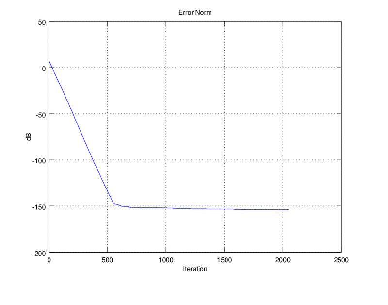
To come up with a frequency domain example of an adaptive LMS filter, you can have an unknown transfer function in parallel with your adaptive filter, where the output of one is subtracted from the other creating an error signal. This is then squared and the steepest descent method is used to find a guess to the LMS error iteratively, after every N point FFT is done and at each frequency. The step size is adjusted to be independent of the amplitude of the input. The result converges nicely. See the derivation in this scratch paper.
Here is a MATLAB or octave file that demonstrates the convergence.
% This is to test the adaptive filter done in the frequency domain.
% It is supposed to converge to an unknown transfer function, Hu.
% Algorithm developed by Rob Frohne 3/22/2012.  Available under GPL.

mu = 1
N = 32
L = 2048;
M = L*N;
e = 0;
Hu = randn(1,N);

H = zeros(size(Hu));

x = 100*randn(1,M);

for k=1:L-1
	X = fft(x(k*N+1:(k+1)*N));
	R = Hu.*X;
	E = R-H.*X;
	H = H + mu*2*E.*conj(X)/(X*X'); % Note: The (X*X') normalizes the
	% step size with respect to the input.
	e = [e,10*log10(norm(H-Hu))];
end

plot(e)
title('Error Norm')
ylabel('dB')
xlabel('Iteration')
Here is the result.
