Class Notes 1-5-2010: Difference between revisions
Jump to navigation
Jump to search
Brian.Roath (talk | contribs) |
No edit summary |
||
| (5 intermediate revisions by 2 users not shown) | |||
| Line 12: | Line 12: | ||
The individual component representation of vector <math> \vec{v} </math> in the x-direction. |
|||
:<math>v_\mathrm{x} = \vec{v} \cdot \mathbf{\hat{i}}</math> |
:<math>v_\mathrm{x} = \vec{v} \cdot \mathbf{\hat{i}}</math> |
||
The two-dimensional example of a vector in its components with the vector designations. |
|||
:<math> \vec{v} = v_\mathrm{x} \mathbf{\hat{i}} + v_\mathrm{y} \mathbf{\hat{j}} </math> |
:<math> \vec{v} = v_\mathrm{x} \mathbf{\hat{i}} + v_\mathrm{y} \mathbf{\hat{j}} </math> |
||
This is the summation used to represent the vector <math> \vec{v} </math> as having as many dimensions as needed to express its full value: |
|||
:<math> \vec{v} = \sum_{i} v_\mathrm{i} \mathbf{\hat{a}}_\mathrm{i} </math> |
:<math> \vec{v} = \sum_{i} v_\mathrm{i} \mathbf{\hat{a}}_\mathrm{i} </math> |
||
:<math> \langle v_x, v_y\rangle</math> |
:<math> \langle v_x, v_y\rangle</math> |
||
This is the equation for finding the distance between the two vectors <math> \vec{u} </math> and <math> \vec{v} </math> who are separated by angle <math> \theta </math>. |
|||
:<math> \ |
:<math> \vec{u} \cdot \vec{v} = |\vec{u}| |\vec{v}| \cos\theta </math> |
||
:<math> \vec{v} \cdot \mathbf{\hat{i}} = v_\mathrm{x} (\mathbf{\hat{i}} \cdot \mathbf{\hat{i}}) + v_\mathrm{y} \mathbf{\hat{j}} \cdot \mathbf{\hat{i}} </math> |
:<math> \vec{v} \cdot \mathbf{\hat{i}} = v_\mathrm{x} (\mathbf{\hat{i}} \cdot \mathbf{\hat{i}}) + v_\mathrm{y} \mathbf{\hat{j}} \cdot \mathbf{\hat{i}} </math> |
||
:<math> \vec{v} \cdot \mathbf{\hat{i}} = v_\mathrm{x} </math> |
:<math> \vec{v} \cdot \mathbf{\hat{i}} = v_\mathrm{x} </math> |
||
:<math> \vec{v} \cdot \mathbf{\hat{a}}_\mathrm{m} = \sum_{i} v_\mathrm{i} \mathbf{\hat{a}}_\mathrm{i} \cdot \mathbf{\hat{a}}_\mathrm{m} = v_\mathrm{m} </math> |
:<math> \vec{v} \cdot \mathbf{\hat{a}}_\mathrm{m} = \sum_{i} v_\mathrm{i} \mathbf{\hat{a}}_\mathrm{i} \cdot \mathbf{\hat{a}}_\mathrm{m} = v_\mathrm{m} </math> |
||
:<math> \delta_\mathrm{i,m} \equiv \begin{cases} 1 & \mbox{if } i = m |
:<math> \delta_\mathrm{i,m} \equiv \begin{cases} 1, & \mbox{if } i = m \\ 0, & \mbox{else} \end{cases}</math> |
||
==Example== |
==Example== |
||
| Line 33: | Line 36: | ||
==External Links== |
==External Links== |
||
* |
*[http://people.wallawalla.edu/~Rob.Frohne/ClassNotes/ENGR351/2010w/Keystone/index.php Class Notes]. |
||
==Authors== |
==Authors== |
||
| Line 39: | Line 42: | ||
Brian Roath |
Brian Roath |
||
==Read By== |
|||
==Reviewed By== |
|||
*[[Gratias, Ryan|Ryan Gratias]] |
|||
Latest revision as of 12:37, 20 January 2010
This article covers the notes given in class on January 5, 2010.
Subjects Covered
1) Linear Systems
2) Functions as Vectors
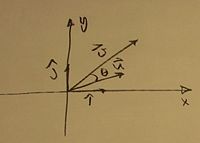
The individual component representation of vector in the x-direction.
The two-dimensional example of a vector in its components with the vector designations.
This is the summation used to represent the vector as having as many dimensions as needed to express its full value:
This is the equation for finding the distance between the two vectors and who are separated by angle .
Example
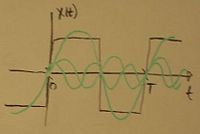
Given function:
1) Use vector analogy
External Links
Authors
Colby Fullerton
Brian Roath


![{\displaystyle x(t)=\sum _{n=1}^{\infty }\left[b_{n}\sin \left(\left({\frac {2\pi n}{T}}\right)t\right)\right]}](https://wikimedia.org/api/rest_v1/media/math/render/svg/1b15fa18143738e6bbe3d2aefb2cc8a5ac979bb7)
![{\displaystyle x(t)\cdot \sin \left({\frac {2\pi mt}{T}}\right)=\sum _{n=1}^{\infty }\left[b_{n}\sin \left(\left({\frac {2\pi n}{T}}\right)t\right)\cdot \sin \left({\frac {2\pi mt}{T}}\right)\right]}](https://wikimedia.org/api/rest_v1/media/math/render/svg/570a428f69ebcdd14e9a313bceea1472ddbf5f67)
