|
|
| Line 20: |
Line 20: |
|
Applying the Laplace Transform to the motion equations and plugging the values of <math>k_1</math>, <math>k_2</math>, <math>k_3</math>, <math>m_1</math>, <math>m_2</math>, <math>x_1(0)</math>, <math>x'1(0)</math>, <math>x_2(0)</math>, and <math>x'_2(0)</math> for this systems, we obtain, |
|
Applying the Laplace Transform to the motion equations and plugging the values of <math>k_1</math>, <math>k_2</math>, <math>k_3</math>, <math>m_1</math>, <math>m_2</math>, <math>x_1(0)</math>, <math>x'1(0)</math>, <math>x_2(0)</math>, and <math>x'_2(0)</math> for this systems, we obtain, |
|
|
|
|
|
:<math>\mathcal{L}[m_1\ddot{x}_1+k_1x_1-k_2(x_2-x_1)]=0</math> |
|
:<math>\mathcal{L}[m_1\ddot{x}_1+k_1x_1-k_2(x_2-x_1)]=m_1[s^2X_1(s)-sx_1(0)-\dot{x}_1(0)]+k_1X_1(s)-k_2(X_2(s)-X_1(s))=0</math> |
|
::<math>m_1[s^2X_1(s)-sx_1(0)-\dot{x}_1(0)]+k_1X_1(s)-k_2(X_2(s)-X_1(s))=0</math> |
|
|
::<math>X_1(s)(m_1s^2+k_1+k_2)=m_1(sx_1(0)-\dot{x}_1(0))+k_2X_2(s)</math> |
|
::<math>X_1(s)(m_1s^2+k_1+k_2)=m_1(sx_1(0)-\dot{x}_1(0))+k_2X_2(s)</math> |
|
::<math>X_1(s)=\dfrac{m_1(sx_1(0)+\dot{x}_1(0))+k_2X_2(s)}{(m_1s^2+k_1+k_2)}</math> |
|
::<math>X_1(s)=\dfrac{m_1(sx_1(0)+\dot{x}_1(0))+k_2X_2(s)}{(m_1s^2+k_1+k_2)}</math> |
| Line 27: |
Line 26: |
|
::<math>X_1(s)=\dfrac{X_2(s)-1}{(s^2+2)}</math> |
|
::<math>X_1(s)=\dfrac{X_2(s)-1}{(s^2+2)}</math> |
|
|
|
|
|
:<math>\mathcal{L}[m_2\ddot{x}_2+k_2(x_2-x_1)+k_3x_2]=0</math> |
|
:<math>\mathcal{L}[m_2\ddot{x}_2+k_2(x_2-x_1)+k_3x_2]=m_2[s^2X_2(s)-sx_2(0)-\dot{x}_2(0)]+k_2(X_2(s)-X_1(s))+k_3X_2(s)=0</math> |
|
::<math>m_2[s^2X_2(s)-sx_2(0)-\dot{x}_2(0)]+k_2(X_2(s)-X_1(s))+k_3X_2(s)=0</math> |
|
|
::<math>X_2(s)(m_2s^2+k_2+k_3)=m_2(sx_2(0)-\dot{x}_2(0))+k_2X_1(s)</math> |
|
::<math>X_2(s)(m_2s^2+k_2+k_3)=m_2(sx_2(0)-\dot{x}_2(0))+k_2X_1(s)</math> |
|
::<math>X_2(s)=\dfrac{m_2(sx_2(0)+\dot{x}_2(0))+k_2X_1(s)}{(m_2s^2+k_2+k_3)}</math> |
|
::<math>X_2(s)=\dfrac{m_2(sx_2(0)+\dot{x}_2(0))+k_2X_1(s)}{(m_2s^2+k_2+k_3)}</math> |
| Line 76: |
Line 74: |
|
|
|
|
|
== Bode Plot == |
|
== Bode Plot == |
|
[[Image:Mass_spring_bode_plot.png|thumb|Figure 3. Bode Diagram.]]The Bode plot can be easily done using a program like Octave or MATLAB. The code is displayed below. From Figure 3 we may notice that the Amplitude vs. Frequency plot for both functions overlaps. On the other hand, the Phase vs. Frequency plot for both functions have opossite magnitudesNotice that both functions overlaps. |
|
[[Image:Mass_spring_bode_plot.png|thumb|Figure 3. Bode Diagram.]]The Bode plot can be easily done using a program like Octave or MATLAB. The code is displayed below. From Figure 3 we may notice that the Amplitude vs. Frequency plot for both functions overlaps. The peak amplitude occurs at about 2 seconds, as well as the phase switching as shown in the Phase vs. Frequency plot. |
|
|
|
|
|
h1=tf([-1],[1 0 3]); |
|
h1=tf([-1],[1 0 3]); |
|
h2=tf([1],[1 0 3]); |
|
h2=tf([1],[1 0 3]); |
|
bode(h1,'b',h2,'r'); |
|
bode(h1,'b',h2,'-.r'); |
|
|
legend('H_1(s)','H_2(s)') |
|
|
grid on; |
|
|
|
|
|
== Magnitude Frequency Response == |
|
== Magnitude Frequency Response == |
Revision as of 01:38, 24 November 2009
Figure 1. Coupled Spring System.
Problem Statement
Derive the system of differential equations describing the straight-line vertical motion of the coupled spring shown in Figure 1. Use Laplace transform to solve the system when  ,
,  , and
, and  ,
,  ,
,  , and
, and  .
.
Solution
At positions  and
and  , the masses
  and
and  are in equilibrium. Thus, the motion equations for and are,

- ∴


- ∴

where  and
and  represent the Newton's Second Law of Motion and
  and
and  represent the net forces acting in the masses.
Laplace Transform
Applying the Laplace Transform to the motion equations and plugging the values of  ,
,  ,
,  , , ,
, , ,  ,
,  ,
,  , and
, and  for this systems, we obtain,
![{\displaystyle {\mathcal {L}}[m_{1}{\ddot {x}}_{1}+k_{1}x_{1}-k_{2}(x_{2}-x_{1})]=m_{1}[s^{2}X_{1}(s)-sx_{1}(0)-{\dot {x}}_{1}(0)]+k_{1}X_{1}(s)-k_{2}(X_{2}(s)-X_{1}(s))=0}](https://wikimedia.org/api/rest_v1/media/math/render/svg/392e87c396fb62f5b82104864e0edf76c8a6f5d9)


![{\displaystyle X_{1}(s)={\dfrac {1(s0+(-1)]+1X_{2}(s)}{(1s^{2}+1+1)}}}](https://wikimedia.org/api/rest_v1/media/math/render/svg/1569d4323a471f35f58c9deed7a415e1d26dfdea)

![{\displaystyle {\mathcal {L}}[m_{2}{\ddot {x}}_{2}+k_{2}(x_{2}-x_{1})+k_{3}x_{2}]=m_{2}[s^{2}X_{2}(s)-sx_{2}(0)-{\dot {x}}_{2}(0)]+k_{2}(X_{2}(s)-X_{1}(s))+k_{3}X_{2}(s)=0}](https://wikimedia.org/api/rest_v1/media/math/render/svg/49aeddc8f5081ddc55dd841a7d07ef8aab4d9903)


Finally, solving for  and
and  yields,


Inverse Laplace Transform
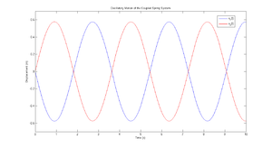
Figure 2. Coupled Spring System Displacement.
First, we recognize that

On the other hand, we identify that  , and so
  . Hence, we fix the expression by multiplying and dividing by
  ,
,
![{\displaystyle x_{1}(t)={\mathcal {L}}^{-1}[X_{1}(s)]={\mathcal {L}}^{-1}\left[{\dfrac {-1}{s^{2}+3}}\right]=-{\dfrac {1}{\sqrt {3}}}{\mathcal {L}}^{-1}\left[{\dfrac {\sqrt {3}}{s^{2}+3}}\right]=-{\dfrac {1}{\sqrt {3}}}sin({\sqrt {3}}t)}](https://wikimedia.org/api/rest_v1/media/math/render/svg/5a32d68f215f452efdbcce10a11e1b233a8fc230)
![{\displaystyle x_{2}=(t){\mathcal {L}}^{-1}[X_{2}(s)]={\mathcal {L}}^{-1}\left[{\dfrac {1}{s^{2}+3}}\right]={\dfrac {1}{\sqrt {3}}}{\mathcal {L}}^{-1}\left[{\dfrac {\sqrt {3}}{s^{2}+3}}\right]={\dfrac {1}{\sqrt {3}}}sin({\sqrt {3}}t)}](https://wikimedia.org/api/rest_v1/media/math/render/svg/19364b5f445eb5a82d33a1d0b3ae49ec90388a72)
A plot of the system displacement is shown on Figure 2.
Initial-Value & Final-Value Theorem
The initial-value and final-value theorem can be useful the finding the behavior of a functionat small and large times respectively. By definition, the Initial-Value Theorem is,

and the Final-Value Theorem is,

Thus, applying both theorems to our the Laplace Transforms,


Bode Plot
The Bode plot can be easily done using a program like Octave or MATLAB. The code is displayed below. From Figure 3 we may notice that the Amplitude vs. Frequency plot for both functions overlaps. The peak amplitude occurs at about 2 seconds, as well as the phase switching as shown in the Phase vs. Frequency plot.
h1=tf([-1],[1 0 3]);
h2=tf([1],[1 0 3]);
bode(h1,'b',h2,'-.r');
legend('H_1(s)','H_2(s)')
grid on;
Magnitude Frequency Response
Convolution
State Equation Model
References


