Problem Statement
Part 1
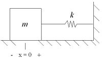
An ideal mass m=10kg is sliding on a surface, attached via an ideal spring k to a rigid wall. The spring is at rest when the mass is centered at x=0. Find the equation of motion that the spring mass system follows if there is an initial f(t) applied. Take friction to be 0.5 between the mass and surface.
As set up, the mass is sitting at x=0 with positive being to the right. Velocity is positive to the right as well.
Part 2
Apply the Initial Value and Final Value Theorems to this problem.
Part 3
Make a bode plot.
Solution
Part 1
First, a FBR:
By Newton's first law:
math>\mathbf{F}=m{a} 21:28, 22 October 2009 (UTC) \Rightarrow 21:28, 22 October 2009 (UTC) \mathbf{f}_m(t)=m\ddot{x}</math>
By Hooke's law:
math>\mathbf{F}=k{x} 21:28, 22 October 2009 (UTC) \Rightarrow 21:28, 22 October 2009 (UTC) \mathbf{f}_k(t)=kx</math>
Now we set up our equation of motion:


We now have a second order differential equation that governs the motion of the mass. If we make our initial conditions equal to zero, we save a few steps. Taking the Laplace transform of both sides gives:


Now that we have the Laplace transform of the differential equation that governs the motion of the spring and mass system, we need to solve for X(s):

Using the idea that the initial position x=0 and velocity is the equivalent of x dot:

Now, let's split it into two parts:

We know from Laplace transforms that:


From this we know that we are going to have two parts to our solution, and sine wave and a cosine wave. We can also tell that:

Once we get the Laplace transform into the correct form, we have:

Now we take the inverse Laplace transform:


Now that we are back in the time domain we just add the two parts together and we have:

So we have found the equation that governs the motion of the spring mass system, all that is left is putting in constants for the variables to find numerical answers for any problem of this type.
Part 2
The Initial Value Theorem states:

So if we plug our equation into this we have:


As expected, the Initial Value Theorem shows us that the initial value is just the initial x value.
The Final Value Theorem States:


It seems as though the Final Value Theorem predicts the final result to be 0. However, in this case, the function is an oscillating one, and the prediction is telling us the average, which is 0. So, in this case the Final Value Theorem is not used to its full potential.
Written by: David Steinweg
Checked by: Nathan Reeves


