Laplace transforms: Critically Damped Motion: Difference between revisions
Jump to navigation
Jump to search
Mark.bernet (talk | contribs) |
Mark.bernet (talk | contribs) |
||
| (30 intermediate revisions by 2 users not shown) | |||
| Line 17: | Line 17: | ||
<math>\text {k=4}\,</math> |
<math>\text {k=4}\,</math> |
||
<math>\text { |
<math>\text {C=2}\,</math> |
||
<math>\text {x(0)=0}\,</math> |
<math>\text {x(0)=0}\,</math> |
||
<math>\dot{x}(0)=-3</math> |
<math>\dot{x}(0)=-3</math> |
||
<math>\text {Therefore the equation representing this system is}\,</math> |
|||
<math>\text {Standard equation: }\,</math> |
|||
<math>m\frac{d^2x}{dt^2}+C\frac{dx}{dt}+khx=0</math> |
|||
===Solving the problem=== |
|||
<math>\text {Therefore the equation representing this system is.}\,</math> |
|||
<math>\frac1 4 \frac{d^2x}{dt^2}=-4x-2\frac{dx}{dt}</math> |
<math>\frac1 4 \frac{d^2x}{dt^2}=-4x-2\frac{dx}{dt}</math> |
||
| Line 33: | Line 39: | ||
<math>\text {Now that we have the equation written in standard form we need to send}\,</math> |
<math>\text {Now that we have the equation written in standard form we need to send}\,</math> |
||
<math>\text {it through the Laplace Transform}\,</math> |
<math>\text {it through the Laplace Transform.}\,</math> |
||
<math>\mathcal{L}[\frac{d^2x}{dt^2}+8\frac{dx}{dt}+16x]</math><br /><br /> |
|||
<math>\text {And we get the equation (after some substitution and simplification)}.\,</math> |
|||
<math>\mathbf s^2 {X}(s)+8\mathbf s{X}(s)+16\mathbf{X}(s)=-3</math><br /><br /> |
|||
<math>\mathbf {X}(s)(s^2+8s+16)=-3</math><br /><br /> |
|||
<math>\mathbf {X}(s)=-\frac{3}{(s+4)^2} </math><br /><br /> |
|||
<math>\text {Now that we have completed the Laplace Transform}\,</math> |
|||
<math>\text {and solved for X(s) we must so an inverse Laplace Transform. }\,</math> |
|||
<math>\mathcal{L}^{-1}[-\frac{3}{(s+4)^2}]</math><br /><br /> |
|||
<math>\text {and we get, by using the table of transforms on p. 515 of the text bokk}\,</math> |
|||
<math>\mathbf {x}(t)=-3te^{-4t}</math><br /><br /> |
|||
<math>\text {So there you have it the equation of a Critically Damped spring mass system.}\,</math> |
|||
==Apply the Initial and Final Value Theorems to find the initial and final values== |
|||
:Initial Value Theorem |
|||
::<math>\lim_{s\rightarrow \infty} sF(s)=f(0)\,</math> |
|||
:Final Value Theorem |
|||
::<math>\lim_{s\rightarrow 0} sF(s)=f(\infty)\,</math> |
|||
===Applying this to our problem=== |
|||
<math>\text {The Initial Value Theorem}\,</math> |
|||
<math>\lim_{s\rightarrow \infty} \mathbf {sX}(s)=-\frac{3}{(s+4)^2}\,</math> |
|||
<math>\lim_{s\rightarrow \infty} \mathbf s{X}(s)=-\frac{3}{(\infty+4)^2}=0\,</math> |
|||
<math>\text {So as you can see the value for the initial position will be 0. }\,</math> |
|||
<math>\text {Which makes sense because the system is initially in equilibrium. }\,</math> |
|||
<math>\text {The Final Value Theorem}\,</math> |
|||
<math>\lim_{s\rightarrow 0} \mathbf s{X}(s)=-\frac{3}{(s+4)^2}\,</math> |
|||
<math>\lim_{s\rightarrow 0} \mathbf s{X}(s)=-\frac{3}{(0+4)^2}=-\frac 3 {16}\,</math> |
|||
<math>\text {This shows the final value to be}\,</math> |
|||
<math>-\frac{3}{16}ft</math> |
|||
<math>\text {Which appears to mean the system will be below equilibrium after a long time. }\,</math> |
|||
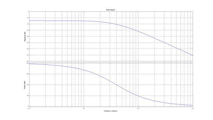
==Bode Plot of the transfer function== |
|||
===Transfer Function=== |
|||
<math>\mathbf {X}(s)=-\frac{3}{(s+4)^2} </math><br /><br /> |
|||
===Bode Plot=== |
|||
<math>\text {This plot is done using the control toolbox in MatLab. }\,</math> |
|||
[[Image:bode.jpg|700px|thumb|left|Fig (1)]] |
|||
==Break Points and Asymptotes== |
|||
<math>\text {A break point is defined by a place in the bode plot where a change occurs.}\,</math> |
|||
<math>\text {To find your break points you must start with a transfer function. }\,</math> |
|||
<math>\text {Transfer Function: }\,</math> |
|||
<math>\mathbf {X}(s)=-\frac{3}{(s+4)^2} </math><br /><br /> |
|||
<math>\text {A break point is located at any value where s = what is being added to it. }\,</math> |
|||
<math>\text {So for this transfer function its at s=4 (that is also the asymptotes location). }\,</math> |
|||
=Convolution= |
|||
<math>\text {The convolution equation is as follows: }\,</math> |
|||
<math> |
|||
x(t)=x_{in}(t) * h(t) = \int_{0}^{t} {x(t_0) \, h(t-t_0) \, dt_0} |
|||
</math> |
|||
<math>\text {It does basically the same thing as the Laplace Transform. }\,</math> |
|||
<math>\text {To start we must inverse transform our transfer function }\,</math> |
|||
<math>\mathbf {X}(s)=-\frac{3}{(s+4)^2} </math><br /><br /> |
|||
<math>\text {Which once more yields: }\,</math> |
|||
<math>\mathbf {x}(t)=-3te^{-4t}</math><br /><br /> |
|||
<math>\text {Then we put this into the convolution integral: }\,</math> |
|||
<math> |
|||
x(t)=x_{in}(t) * h(t) = \int_{0}^{t} {-3(t-t_0)e^{-4t-t_0} \, dt_0} |
|||
</math> |
|||
<math>\text {Which once more yeilds: }\,</math> |
|||
<math>\mathbf {x}(t)=(-cte^{-4t})</math><br /><br /> |
|||
<math>\text {Not exactly the same but remember initial conditions arnt used}\,</math> |
|||
=State Space= |
|||
<math>\text {Using state equatons is just another way to solve a system modeled by an ODE }\,</math> |
|||
<math>\text {First we need to add an applied force so u(t)=2N }\,</math> |
|||
<math>m=\frac{8}{32}=\frac1 4 slugs</math> |
|||
<math>\text {k=4}\,</math> |
|||
<math>\text {C=2}\,</math> |
|||
<math>\text {x(0)=0}\,</math> |
|||
<math>\dot{x}(0)=-3</math> |
|||
<math>\ddot{x}(0)=0</math> |
|||
<math>\begin{bmatrix} \dot{x} \\ \ddot{x} \end{bmatrix}=\begin{bmatrix} 0 & 1 \\ -k/m & -C/m \end{bmatrix} \begin{bmatrix} x \\ \dot{x} \end{bmatrix} + \begin{bmatrix} 0 \\ 1/m \end{bmatrix}u(t)</math> |
|||
--- |
|||
Written By: Mark Bernet |
|||
Error Checked By: Greg Peterson |
|||
<math>\mathcal{L}_s\frac{d^2x}{dt^2}+8\frac{dx}{dt}+16x</math><br /><br /> |
|||
Latest revision as of 16:58, 18 November 2009
Using the Laplace Transform to solve a spring mass system that is critically damped
Problem Statement
An 8 pound weight is attached to a spring with a spring constant k of 4 lb/ft. The spring is stretched 2 ft and rests at its equilibrium position. It is then released from rest with an initial upward velocity of 3 ft/s. The system contains a damping force of 2 times the initial velocity.
Solution
Things we know
Solving the problem
Apply the Initial and Final Value Theorems to find the initial and final values
- Initial Value Theorem
- Final Value Theorem
Applying this to our problem
Bode Plot of the transfer function
Transfer Function
Bode Plot
==Break Points and Asymptotes==
Convolution
State Space
---
Written By: Mark Bernet
Error Checked By: Greg Peterson


![{\displaystyle {\mathcal {L}}[{\frac {d^{2}x}{dt^{2}}}+8{\frac {dx}{dt}}+16x]}](https://wikimedia.org/api/rest_v1/media/math/render/svg/9223069732914f355e25cc2ee4ac7c6e4b58e571)


![{\displaystyle {\mathcal {L}}^{-1}[-{\frac {3}{(s+4)^{2}}}]}](https://wikimedia.org/api/rest_v1/media/math/render/svg/1dfc431d35b72b5580c7bbfb1bd441dfdfcb2394)


