Laplace transforms: Under-damped Mass-Spring System on an Incline

Brandon.plubell 05:44, 26 October 2009 (UTC)

Under-Damped Mass-Spring System on an Incline

Part 1 - Use Laplace Transformations

Problem Statement

Find the equation of motion for the mass in the system subjected to the forces shown in the Free Body Diagram (FBD). The inclined surface is coated in SAE 30 oil.

Initial Conditions and Values

• A is the area of the box in contact with the surface
• g is the gravitational acceleration field constant
• b_t is the thickness of the fluid covering the inclined surface
• μ is the viscosity constant of the fluid;
• m is the mass of the box
• k is the spring constant

$A={\frac {1}{4}}m^{2}$

$g=9.81{\frac {m}{s^{2}}}$

$b_{t}=1mm{\frac {}{}}$

$\mu =0.06{\frac {N\cdot s}{m^{2}}}$

$m=45kg{\frac {}{}}$

$k=200{\frac {N}{m}}$

$\theta =30^{\circ }{\frac {}{}}$

Let the initial conditions be:

$x(0)=-0.5m{\frac {}{}}$

${\dot {x}}(0)=0{\frac {m}{s}}$

Force Equations

The sum of the moments in the x direction yields the equatiom

$+\swarrow \sum F_{x}=m{\ddot {x}}$

$\Rightarrow \ m{\ddot {x}}=F_{s}+F_{f}+mg\sin \theta$

Where

$F_{s}=-k\,x$

$F_{f}=-{\frac {\mu \,A}{b_{t}}}\,{\dot {x}}$

To make the algebra easier, let

$\lambda ={\frac {\mu \,A}{b_{t}}}$

Then, from the sum of forces equation:

$m\,{\ddot {x}}+\lambda \,{\dot {x}}+k\,x=mg\sin \theta$

$\Rightarrow \ {\ddot {x}}+{\frac {\lambda }{m}}\,{\dot {x}}+{\frac {k}{m}}\,x=g\sin \theta$

Laplace Transform

${\mathcal {L}}\left\{{\ddot {x}}+{\frac {\lambda }{m}}\,{\dot {x}}+{\frac {k}{m}}\,x\right\}={\mathcal {L}}\left\{g\sin \theta \right\}$

$\Rightarrow \ s^{2}\,X(s)-s\,x(0)-{\dot {x}}(0)+{\frac {\lambda }{m}}\,s\,X(s)-{\frac {\lambda }{m}}\,x(0)+{\frac {k}{m}}\,X(s)=g\sin \theta \,\left({\frac {1}{s}}\right)$

$\Rightarrow \ X(s)\left(s^{2}+{\frac {\lambda }{m}}\,s+{\frac {k}{m}}\right)=g\sin \theta \,\left({\frac {1}{s}}\right)+s\,x(0)+{\dot {x}}(0)+{\frac {\lambda }{m}}\,x(0)$

If we let $x(0){\text{ and }}{\dot {x}}(0)$ be 0 and rearrange the equation,

${\frac {X(s)}{X_{in}(s)}}={\frac {X(s)}{g\sin \theta \left({\frac {1}{s}}\right)}}=H(s)$

$\Rightarrow H(s)={\frac {1}{s^{2}+{\frac {\lambda }{m}}\,s+{\frac {k}{m}}}}$

The above is the transfer function that will be used in the Bode plot and can provide valuable information about the system.

$X(s)=g\sin \theta \left({\frac {1}{s}}\right)\left({\frac {1}{s^{2}+{\frac {\lambda }{m}}\,s+{\frac {k}{m}}}}\right)+x(0)\,\left({\frac {s}{s^{2}+{\frac {\lambda }{m}}\,s+{\frac {k}{m}}}}\right)+\left({\dot {x}}(0)+{\frac {\lambda }{m}}\,x(0)\right)\,\left({\frac {1}{s^{2}+{\frac {\lambda }{m}}\,s+{\frac {k}{m}}}}\right)$

Inverse Laplace Transform

Since the Laplace Transform is a linear transform, we need only find three inverse transforms. All of the these have complex roots, since ${\left({\frac {\lambda }{m}}\right)}^{2}<4\,{\frac {\lambda }{m}}$. Because I am not yet comfortable finding the inverse with complex roots by hand, I used a laplace transform program for the TI-89.

${\mathcal {L}}^{-1}\left\{{\frac {1}{s\left(s^{2}+{\frac {\lambda }{m}}\,s+{\frac {k}{m}}\right)}}\right\}=e^{{\frac {-1}{6}}\,t}\,\left[{\frac {-9}{40}}\cos {\left({\frac {{\sqrt {159}}\,t}{6}}\right)}-{\frac {3\,{\sqrt {159}}}{2120}}\,\sin {\left({\frac {{\sqrt {159}}\,t}{6}}\right)}\right]+{\frac {9}{40}}$

${\mathcal {L}}^{-1}\left\{{\frac {s}{s^{2}+{\frac {\lambda }{m}}\,s+{\frac {k}{m}}}}\right\}=e^{{\frac {-1}{6}}\,t}\,\left[\cos {\left({\frac {{\sqrt {159}}\,t}{6}}\right)}-{\frac {\sqrt {159}}{159}}\,\sin {\left({\frac {{\sqrt {159}}\,t}{6}}\right)}\right]$

${\mathcal {L}}^{-1}\left\{{\frac {1}{s^{2}+{\frac {\lambda }{m}}\,s+{\frac {k}{m}}}}\right\}=e^{{\frac {-1}{6}}\,t}\,\left[{\frac {2\,{\sqrt {159}}}{53}}\,\sin {\left({\frac {{\sqrt {159}}\,t}{6}}\right)}\right]$

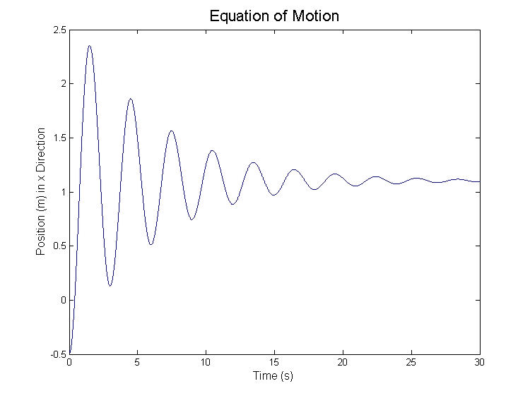
Equation of Motion

Putting it all back together again gives,

$x(0)=g\,\sin {\theta }\,\left(e^{{\frac {-1}{6}}\,t}\,\left[{\frac {-9}{40}}\cos {\left({\frac {{\sqrt {159}}\,t}{6}}\right)}-{\frac {3\,{\sqrt {159}}}{2120}}\,\sin {\left({\frac {{\sqrt {159}}\,t}{6}}\right)}\right]+{\frac {9}{40}}\right)$

$+\,x(0)\,\left(e^{{\frac {-1}{6}}\,t}\,\left[\cos {\left({\frac {{\sqrt {159}}\,t}{6}}\right)}-{\frac {\sqrt {159}}{159}}\,\sin {\left({\frac {{\sqrt {159}}\,t}{6}}\right)}\right]\right)$

$+\left({\dot {x}}(0)+{\frac {\lambda }{m}}\,x(0)\right)\,\left(e^{{\frac {-1}{6}}\,t}\,\left[{\frac {2\,{\sqrt {159}}}{53}}\,\sin {\left({\frac {{\sqrt {159}}\,t}{6}}\right)}\right]\right)$

It is useful to have the equation in the form given above because $x(0){\text{ , }}{\dot {x}}(0){\text{ , }}\theta {\text{ , and even }}g$ can be varied and still give accurate results. The Matlab (or Octave) script below can be edited as described. Take note! $\lambda {\text{ (and all that depend on it), }}m{\text{ , and }}k$ cannot be altered (else the inverse Laplace is false)!

Matlab Script

Part 2 - Final and Initial Value Theorems

Initial Value Theorem

As was derived in class, there are two theorems that relate the initial and final values (in this case positions) of the output functions in the t domain with the output function in the s domain. In a case such as this, in which the initial values are given, the initial value theorem is just a check.

$\lim _{s\to \infty }{s\,X(s)}=x(0)$

Taking the limit of $s\,X(s)$ gives

$\Rightarrow \ \left(g\sin {\theta }\right)\,(0)+\left(x(0)\right)\,(1)+\left({\dot {x}}(0)+{\frac {\lambda }{m}}\,x(0)\right)\,(0)=x(0)$

$\Rightarrow \ x(0)=x(0){\frac {}{}}$

Final Value Theorem

The Final Value Theorem is a very useful tool that will show what the final value of the output function (as $t\to \infty$), which in this case is the final position of the block. Notice that it is not the unstretched length of the spring (else $x(\infty )=0$). It is also of interest to note that only the input function comes into play here, as all the others go to zero, and is not dependent on the initial position or velocity.

$\lim _{s\to 0}{s\,X(s)}=x(\infty )$

$\Rightarrow \ \left(g\sin {\theta }\right)\,({\frac {m}{k}})+\left(x(0)\right)\,(0)+\left({\dot {x}}(0)+{\frac {\lambda }{m}}\,x(0)\right)\,(0)=x(\infty )$

$\Rightarrow \ x(\infty )={\frac {m\,g}{k}}\sin {\theta }=1.104m$

Which can be seen in the plot in Equation of Motion section.

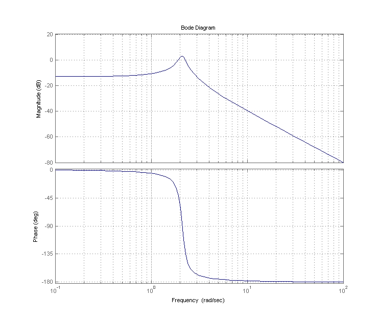
Part 3 - Bode Plot

The bode plot shows useful information about the system we are analyzing. It has only to do with the transfer function, which means that it does not change based upon the input. However, it can show what a given frequency of a harmonic input will do to the output. For my example, it can be seen that at about $2rad/s$ there is a rise in the magnitude of the transfer function. If it were hit with a corresponding frequency by an input function, it could have very larg oscillations.