How a CD player works - HW8: Difference between revisions
Max.Woesner (talk | contribs) No edit summary |
Max.Woesner (talk | contribs) No edit summary |
||
| Line 14: | Line 14: | ||
The discrete function of time <math> x(nT)\!</math> can be expressed mathematically as <math>\sum_{n=-\infty}^\infty x(nT) \delta (t-nT) \!</math>. It might look like this.<br> |
The discrete function of time <math> x(nT)\!</math> can be expressed mathematically as <math>\sum_{n=-\infty}^\infty x(nT) \delta (t-nT) \!</math>. It might look like this.<br> |
||
[[Image:x_discrete.jpg]]<br> |
[[Image:x_discrete.jpg]]<br> |
||
In the frequency domain, the function can be expressed as <math>\frac{1}{T}\sum_{n=-\infty}^\infty X\bigg(f-\frac{n}{T}\bigg)</math> and would look like this.<br> |
In the frequency domain, the function can be expressed either as <math>\frac{1}{T}\sum_{n=-\infty}^\infty X\bigg(f-\frac{n}{T}\bigg)</math> or <math> \sum_{n=-\infty}^\infty x(nT)e^{-j2\pi fnT} \!</math> and would look like this.<br> |
||
[[Image:x_frequency2.jpg]]<br> |
[[Image:x_frequency2.jpg]]<br> |
||
Oversampling can be used to create a smoother discrete function by filling in the gaps with more data points. For example, 8x oversampling, which is fairly common, would decrease the sampling period by a factor of eight, giving us a more accurate function of the original signal. For this page, however, we will focus on 1x oversampling. While no additional data points are added with 1x oversampling, the same process can be used as with 8x oversampling, creating a digital filter. <br><br> |
Oversampling can be used to create a smoother discrete function by filling in the gaps with more data points. For example, 8x oversampling, which is fairly common, would decrease the sampling period by a factor of eight, giving us a more accurate function of the original signal. For this page, however, we will focus on 1x oversampling. While no additional data points are added with 1x oversampling, the same process can be used as with 8x oversampling, creating a digital filter. <br><br> |
||
| Line 40: | Line 40: | ||
<math> \sum_{l=-\infty}^\infty y(lT) \delta (t-lT) * p(t) = \sum_{l=-\infty}^\infty y(lT) p(t-lT)\!</math><br><br> |
<math> \sum_{l=-\infty}^\infty y(lT) \delta (t-lT) * p(t) = \sum_{l=-\infty}^\infty y(lT) p(t-lT)\!</math><br><br> |
||
This convolution gives us a step function, such as the one below.<br> |
This convolution gives us a step function, such as the one below.<br> |
||
The frequency equivalent of <math> p(t) \!</math>, or <math> P(f) \!</math>, can be expressed as <math> P(f) = T sin(fT)\!</math> and will look something like this.<br> |
|||
Since the equivalent to convolution in time is multiplication in frequency, we will multiply <math> P(f)\!</math> by <math>\sum_{n=-\infty}^\infty x(nT)e^{-j2\pi fnT}\!</math>, or <br> |
|||
<math>T sin(fT) \cdot \sum_{n=-\infty}^\infty x(nT)e^{-j2\pi fnT} \!</math>. It would look like this.<br> |
|||
Revision as of 09:14, 29 October 2009
Max Woesner
Homework #8 - How a CD player works
This page describes how a CD player works with no oversampling but with digital filtering, i.e. 1x oversampling.
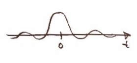
When music for an audio CD is produced, the music has infinite data points and can be expressed as as a continuous function of time, or , such as the one shown below.
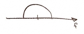
In the frequency domain, the signal looks like this.
Since a CD has a finite amount of storage space, it would be impossible to store on a CD. To solve this problem, the data is sampled at periodic intervals, creating a discrete function of time , where is and integer and is the period between samples.
The sample rate . Since human hearing can typically range from 20 Hz to 22 kHz, we want to sample at a rate greater than twice the highest frequency, or 44 kHz.
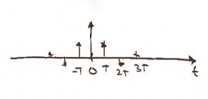
The discrete function of time can be expressed mathematically as . It might look like this.
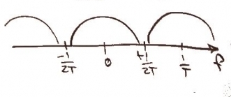
In the frequency domain, the function can be expressed either as or and would look like this.
Oversampling can be used to create a smoother discrete function by filling in the gaps with more data points. For example, 8x oversampling, which is fairly common, would decrease the sampling period by a factor of eight, giving us a more accurate function of the original signal. For this page, however, we will focus on 1x oversampling. While no additional data points are added with 1x oversampling, the same process can be used as with 8x oversampling, creating a digital filter.
To do this, we want to convolve our discrete function by a new function defined as , where is the oversampling rate.
In this case, , so
. Since we are using 1x oversampling, the function won't look any different than the original discrete function.

The frequency response of this is , which looks like this.
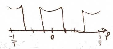
The convolution of our discrete function and can be expressed mathematically as
Let , so , so
Let us define as the function , so
. It would look something like this.
The frequency equivalent would be . It can also be expressed as
, or
This is what it would look like.
Now we are ready to convolve our function with a function , which is done by the D/A converter in a CD player.
and would look like this
This convolution gives us a step function, such as the one below.
The frequency equivalent of , or , can be expressed as and will look something like this.
Since the equivalent to convolution in time is multiplication in frequency, we will multiply by , or
. It would look like this.


![{\displaystyle H(f)={\mathcal {F}}{\Bigg [}\sum _{m=-M}^{M}h(mT)\,\delta (t-mT){\Bigg ]}=\sum _{m=-M}^{M}h(mT)e^{-j2\pi fmT}}](https://wikimedia.org/api/rest_v1/media/math/render/svg/88d643f8ba3becbff42183d9fa5ef346659b4ab4)


![{\displaystyle x(t)*h(t)\ =\sum _{n=-\infty }^{\infty }\sum _{m=-M}^{M}x[(l-m)T]h(mT)\,\delta (t-lT)\!}](https://wikimedia.org/api/rest_v1/media/math/render/svg/c54408b2948da1b33b46d34355249545227181be)
![{\displaystyle \sum _{m=-M}^{M}x[(l-m)T]h(mT)\!}](https://wikimedia.org/api/rest_v1/media/math/render/svg/0503bf750025265742c8a739768729992fdba0fd)


