Using the DFT: Difference between revisions
Jump to navigation
Jump to search
No edit summary |
No edit summary |
||
| Line 5: | Line 5: | ||
Script for matlab: |
Script for matlab: |
||
<pre> |
|||
clear all; |
clear all; |
||
t=0:.01:1; |
t=0:.01:1; |
||
T=0.20; |
T=0.20; |
||
ts=0:T:1; |
ts=0:T:1; |
||
f1=2; |
f1=2; |
||
f2=1/0.125; |
f2=1/0.125; |
||
x = sin(2*pi*3*t); %this is the function |
x = sin(2*pi*3*t); %this is the function |
||
plot(t,x); % plot the original signal |
plot(t,x); % plot the original signal |
||
X = fft(x); % take the DFT |
X = fft(x); % take the DFT |
||
pause (2); |
pause (2); |
||
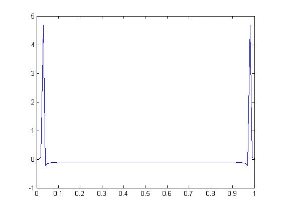
plot (t,X); %plot the DFT of the signal |
plot (t,X); %plot the DFT of the signal |
||
</pre> |
|||

