Using the DFT: Difference between revisions
Jump to navigation
Jump to search
New page: Script for matlab: clear all; t=0:.01:1; T=0.20; ts=0:T:1; f1=2; f2=1/0.125; x = sin(2*pi*3*t); %this is the function plot(t,x); % plot the original signal X = fft(x); % take the DFT pause... |
No edit summary |
||
| (10 intermediate revisions by 2 users not shown) | |||
| Line 1: | Line 1: | ||
This is what we get when we sample the signal at 3Hz | |||
[[Image:hw13_1.jpg]] | |||
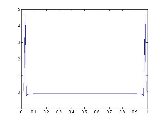
Taking the original signal <math>sin(2*pi*t)</math> and applying the DFT we get this graph: | |||
[[Image:Signals-13.jpg]] | |||
Now taking the DFT of this sampled signal, we get a graph like this: | |||
[[Image:hw13_2.jpg]] | |||
Script for matlab: | Script for matlab: | ||
clear all; | clear all; | ||
t=0:.01: | |||
T= | t=0:.01:2; | ||
ts=0:T: | |||
T=1/3; | |||
ts=0:T:2; | |||
f1=2; | f1=2; | ||
f2=1/0.125; | f2=1/0.125; | ||
x = sin(2*pi* | |||
plot(t, | x = sin(2*pi*ts); %this is the function | ||
plot(ts,sin(2*pi*ts),'r-',t,sin(2*pi*t)); % plot the original signal and the signal sampled at 3Hz | |||
X = fft(x); % take the DFT | X = fft(x); % take the DFT | ||
pause (2); | pause (2); | ||
plot (t,X); %plot the DFT of the signal | |||
plot (ts,X); %plot the DFT of the signal sampled at 3Hz | |||
pause (4); | |||
x=sin(2*pi*t); | |||
plot(t,x); | |||
pause(2); | |||
X = fft(x); | |||
plot(t,X); %plot the DFT of the original signal | |||
Latest revision as of 11:18, 27 November 2007
This is what we get when we sample the signal at 3Hz
Taking the original signal and applying the DFT we get this graph:
Now taking the DFT of this sampled signal, we get a graph like this:
Script for matlab:
clear all;
t=0:.01:2;
T=1/3;
ts=0:T:2;
f1=2;
f2=1/0.125;
x = sin(2*pi*ts); %this is the function
plot(ts,sin(2*pi*ts),'r-',t,sin(2*pi*t)); % plot the original signal and the signal sampled at 3Hz
X = fft(x); % take the DFT
pause (2);
plot (ts,X); %plot the DFT of the signal sampled at 3Hz
pause (4);
x=sin(2*pi*t);
plot(t,x);
pause(2);
X = fft(x);
plot(t,X); %plot the DFT of the original signal
