Homework Eight: Difference between revisions
No edit summary |
No edit summary |
||
| Line 27: | Line 27: | ||
[[Image:x_discrete_a.jpg |thumb|center|upright=2|Figure 7: Original function, x(nT), convolved with the FIR filter, g(t)]] |
[[Image:x_discrete_a.jpg |thumb|center|upright=2|Figure 7: Original function, x(nT), convolved with the FIR filter, g(t)]] |
||
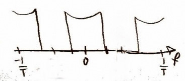
[[Image:x_frequency4a.jpg |thumb|center|upright=2|Figure 8: Original function multiplied by the FIR filter in frequency domain]] |
[[Image:x_frequency4a.jpg |thumb|center|upright=2|Figure 8: Original function multiplied by the FIR filter in frequency domain]] |
||
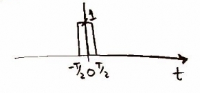
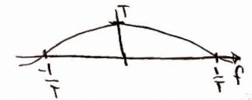
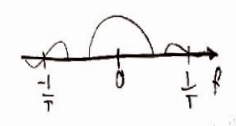
At this point, we are ready to send the audio signal through a D/A converter -- which will essentially convolve the signal with a pulse function, say p(t). The pulse function is shown in the time domain ['''Figure 9'''] and the frequency domain ['''Figure 10'''] |
|||
[[Image:p_t.jpg |thumb|center|upright=2|Figure 7: Pulse function in the time domain, p(t)]] |
|||
[[Image:P_f.jpg |thumb|center|upright=2|Figure 8: Pulse function in the frequency domain, P(f)]] |
|||
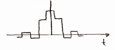
And the convolution of the pulse function with the above FIR filtered function in the time domain ['''Figure 11'''] and the frequency domain ['''Figure 12'''] is shown below |
|||
[[Image:x_step.jpg |thumb|center|upright=2|Figure 7: FIR filtered function convolved with p(t) (time)]] |
|||
[[Image:x_frequency5.jpg |thumb|center|upright=2|Figure 8: FIR filtered function multiplied with P(f) (frequency)]] |
|||
Revision as of 19:42, 8 November 2009
How does a CD player work with no oversampling, but digital filtering (1x oversampling)?
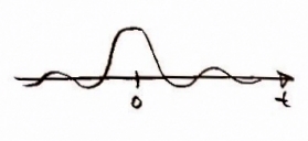
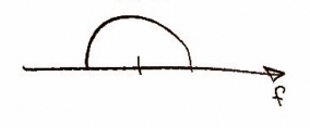
Recall that when the audio for a music CD is produced it has an infinite amount of data points which can be expressed as in the time domain [Figure 1] and in the frequency domain [Figure 2].
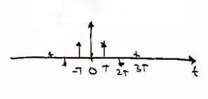
When one wants to store the data of (i.e. reading the data onto a CD in this case) an infinite number of data points is not ideal -- in fact, it is impossible. Therefore, we must sample the data at the (typical) rate of . This will give us a periodic function which we will call is the sampling period. It is common to allow a sampling rate of twice the frequency at which a human can hear (i.e. 2 x 22 kHz) -- that means, kHz.
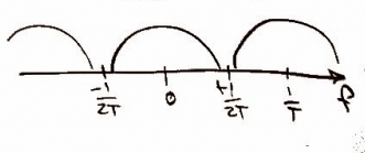
Recall from class that in order to sample the original function, , we need to use a delta function. In other words, the continuous function of can be written as [Figure 3]. As one may expect, in the frequency domain we should get the same plot as in Figure 2, but it should repeat. In the frequency domain, this can be expressed as [Figure 4].
As one may suspect, in order to get a more accurate function you must take more data points -- in other words, a higher sampling rate (i.e. 2x, 8x, etc. oversampling) leads to a more accurate collection of data. For this case, we are asked to looked a digital sampling, or 1x oversampling. In order to accomplish this, we will convolve our function from above with a Finite Impulse Response filter (FIR filter). Let's call the FIR g(t) and define it as where is the oversampling rate. In our case . Because we are dealing with digital sampling, the convolution will result in the original function [Figure 5]. It is fairly easy to see that in the frequency domain, the FIR filter will be expressed as [Figure 6].
As we know, convolution in the time domain results in multiplication in the frequency domain. The results of the convolution and multiplication of the before mentioned FIR filter (time, frequency) are shown below:
At this point, we are ready to send the audio signal through a D/A converter -- which will essentially convolve the signal with a pulse function, say p(t). The pulse function is shown in the time domain [Figure 9] and the frequency domain [Figure 10]
And the convolution of the pulse function with the above FIR filtered function in the time domain [Figure 11] and the frequency domain [Figure 12] is shown below


