8 - 1x oversampling

Write a section on the Wiki about how a CD player works with no oversampling, but digital filtering (1x oversampling)

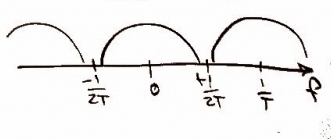
First we sample the data at $f_{s}={\frac {1}{T}}$ to get the data in digital form and when you use the impulse function in time the frequency repeats forever as shown

                                 Sample $f_{s}={\frac {1}{T}}\Longrightarrow$

Where the impulse function with respect to time = $\sum _{n=-\infty }^{\infty }x(nt)\delta (t-nT)$
and ${\frac {1}{T}}\sum _{n=-\infty }^{\infty }X(f-{\frac {n}{T}})$ in the frequency domain.

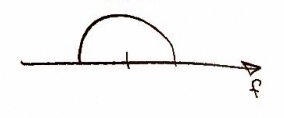
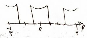
Now that we have the data in the computer we want to convolve it with another impulse function $\sum _{m=-M}^{M}h({\frac {mT}{n}})\delta (t-{\frac {mT}{n}})$ in the time domain. This is where more that 1x oversampling would occur replace n for nx oversampling, but in our case we use n = 1. Doing this convolution we can also shape our frequency when you convolve in time it multiplies in frequency. So we pick a frequency function $\sum _{m=-M}^{M}h({\frac {mT}{n}})e^{-j2\pi fm{\frac {T}{n}}}$ to multiply by so our frequency won't overlap later and help compensate for losses in high frequencies from the D/A converter and low-pass filter. Example the frequency function is.

$\sum _{m=-M}^{M}h({\frac {mT}{n}})e^{-j2\pi fm{\frac {T}{n}}}\Longrightarrow$

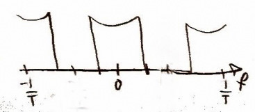
Now doing the convolution/multiplication yields.
The time domain stays the same with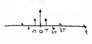

But frequency

x

=

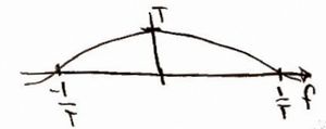
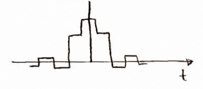
Now it is time to convolve our time function with a pulse function p(t) and thereby multiply our frequency by its pulse equivalent P(f) = Tsin(fT) giving us
*=
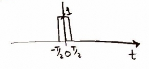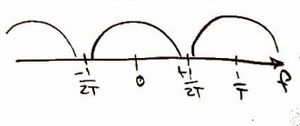
And in frequency

x

=

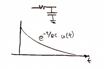
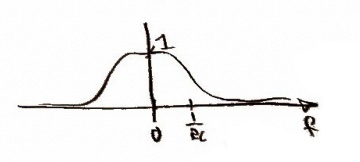
Notice that by pre-emphasizing the high frequencies we get close to what the original function was in the frequency domain. Now the last step before sending the data out to speakers we convolve the time domain function with a simple low-pass filter to smooth the edges of the function and bring the frequency function even closer to its original state giving us a final beautiful sound through our speakers.

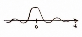
example time domain low-pass filter

example frequency domain low-pass filter