HW8: Difference between revisions
No edit summary |
No edit summary |
||
| (One intermediate revision by the same user not shown) | |||
| Line 5: | Line 5: | ||
'''Solution''' | '''Solution''' | ||
CD players are used to play audio files and although these are limited we can look at any non periodic signal as periodic with an infinite period. We can represent this signal, x(t) as such in the time domain and X(f) in the frequency domain. | CD players are used to play audio files and although these are limited we can look at any non periodic signal as periodic with an infinite period. We can represent this signal, x(t) as such in the time domain and X(f) in the frequency domain. | ||
[[Image:x_continuous3.jpg]] [[Image:x_frequency1b.jpg]] | [[Image:x_continuous3.jpg]] [[Image:x_frequency1b.jpg]] | ||
In order to take the signal and read it digitally we must sample it. This gives us data points creating a discrete function of time <math> x(nT)\!</math>, where <math> n\!</math> is and integer and <math> T\!</math> is the period between samples. We use a frequency of 44 kHz as it is twice the frequency at which a human can hear (i.e. 2 x 22 kHz) -- that means, <math>\scriptstyle f_{s} = 44</math> kHz. Mathematically sampling is represented by multiplying x(t) with the delta function which results in a convolution with X(f). | In order to take the signal and read it digitally we must sample it. This gives us data points creating a discrete function of time <math> x(nT)\!</math>, where <math> n\!</math> is and integer and <math> T\!</math> is the period between samples. We use a frequency of 44 kHz as it is twice the frequency at which a human can hear (i.e. 2 x 22 kHz) -- that means, <math>\scriptstyle f_{s} = 44</math> kHz. Mathematically sampling is represented by multiplying x(t) with the delta function which results in a convolution with X(f). | ||
| Line 32: | Line 32: | ||
Lets call these p(t) and P(f). | Lets call these p(t) and P(f). | ||
We can now convolve the sampled signal with the pulse signal to produce our digital signal. In the frequency domain we get a multiplication once again. | |||
[[image:x_step.jpg]] [[image:x_frequency5.jpg]] | |||
Mathematically these are: <math>\sum_{n=-\infty}^{\infty}x(nT)p(t-nT)</math> and <math>P(f)\left[ \sum_{n=-\infty}^{\infty}x(nT)e^{-j2 \pi fnT} \right]</math>, respectively. | |||
Finally we output the signal. In order to get a smooth sound we finally send the signal through a low pass filter. This will return us to our original signal, sweet sounding tunes. | |||
[[image:lowpass_g_t.jpg]] [[image:lowpass_G_f.jpg]] | |||
Graphically we can see that the digital wave will become more analog and the frequency response will eliminate everything outside the desired frequencies. | |||
[[Image:x_continuous3.jpg]] [[Image:x_frequency1b.jpg]] | |||
Thank you to max for most of the images. | |||
Latest revision as of 01:26, 25 November 2009
Problem Statement
Write a section describing how a CD player works with out oversampling but with digital filtering (1x oversampling)
Solution
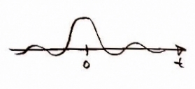
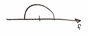
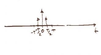
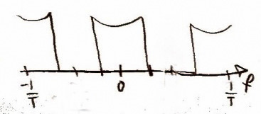
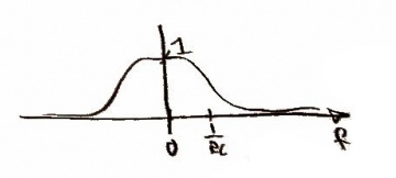
CD players are used to play audio files and although these are limited we can look at any non periodic signal as periodic with an infinite period. We can represent this signal, x(t) as such in the time domain and X(f) in the frequency domain.
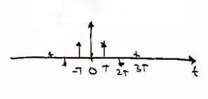
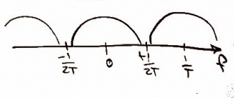
In order to take the signal and read it digitally we must sample it. This gives us data points creating a discrete function of time , where is and integer and is the period between samples. We use a frequency of 44 kHz as it is twice the frequency at which a human can hear (i.e. 2 x 22 kHz) -- that means, kHz. Mathematically sampling is represented by multiplying x(t) with the delta function which results in a convolution with X(f).
Represented as: and respectively.
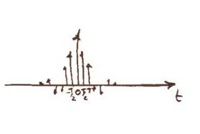
This type of sampling can result in aliasing. This is prevented by oversampling represented on CD players and other media devices as Nx for N times oversampling. It is commonly seen at 8 or 16 and my latest player had it at 52. For this particular assignment we were asked to look at digital filtering but we can accommodate for any oversampling with the variable 'p'. We will use a FIR filter for this. It can be represented graphically as:
and mathematically as: and .
When we run the signal through this filter we multiply it mathematically in the time domain. In the frequency domain this will look like convolution.
x(t)*g(t) and X(f)G(f)
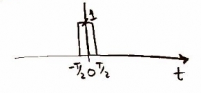
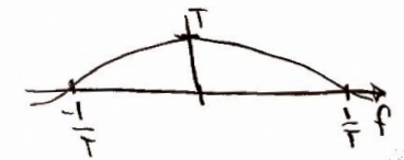
Next we send the signal through a D/A converter. This allows the computer inside the CD player to read the signal information. Graphically this is just a step up and step down a half the period long, known as a pulse function.
Lets call these p(t) and P(f).
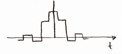
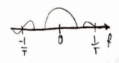
We can now convolve the sampled signal with the pulse signal to produce our digital signal. In the frequency domain we get a multiplication once again.
Mathematically these are: and , respectively.
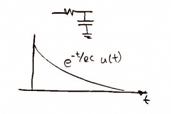
Finally we output the signal. In order to get a smooth sound we finally send the signal through a low pass filter. This will return us to our original signal, sweet sounding tunes.
Graphically we can see that the digital wave will become more analog and the frequency response will eliminate everything outside the desired frequencies.
Thank you to max for most of the images.
