Coupled Oscillator: Jonathan Schreven

Problem

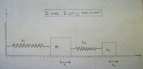
In this problem we will explore the solution of a double spring/mass system under the assumption that the blocks are resting on a smooth surface. Here's a picture of what we are working with.

Equations of Equilibrium

Using F=ma we can then find our four equations of equilibrium.

Equation 1

${\begin{alignedat}{3}F&=ma\\F&=m{\ddot {x}}\\-k_{1}x_{1}-k_{2}(x_{1}x_{2})&=m_{1}{\ddot {x_{1}}}\\-{k_{1}x_{1} \over {m_{1}}}-{k_{2}(x_{1}-x_{2}) \over {m_{1}}}&=m_{1}{\ddot {x_{1}}}\\-{k_{1}x_{1} \over {m_{1}}}-{k_{2}(x_{1}-x_{2}) \over {m_{1}}}&={\ddot {x_{1}}}\\-{k_{1}+k_{2} \over {m_{1}}}x_{1}+{k_{2} \over {m_{1}}}x_{2}&={\ddot {x_{1}}}\\\end{alignedat}}$

Equation 2

${\begin{alignedat}{3}F&=ma\\F&=m{\ddot {x}}\\-k_{2}(x_{2}-x_{1})&=m_{2}{\ddot {x_{2}}}\\{-k_{2}(x_{2}-x_{1}) \over {m_{2}}}&={\ddot {x_{2}}}\\-{k_{2} \over {m_{2}}}x_{2}+{k_{2} \over {m_{2}}}x_{1}&={\ddot {x_{2}}}\\\end{alignedat}}$

Equation 3

${\dot {x_{1}}}={\dot {x_{1}}}$

Equation 4

${\dot {x_{2}}}={\dot {x_{2}}}$

Now we can put these four equations into the state space form.

${\begin{bmatrix}{\dot {x_{1}}}\\{\ddot {x_{1}}}\\{\dot {x_{2}}}\\{\ddot {x_{2}}}\end{bmatrix}}={\begin{bmatrix}0&1&0&0\\-{(k_{1}+k_{2}) \over {m_{1}}}&0&{k_{2} \over {m_{1}}}&0\\0&0&0&1\\{k_{2} \over {m_{2}}}&0&-{k_{2} \over {m_{2}}}&0\end{bmatrix}}{\begin{bmatrix}{x_{1}}\\{\dot {x_{1}}}\\{x_{2}}\\{\dot {x_{2}}}\end{bmatrix}}+{\begin{bmatrix}0\\0\\0\\0\end{bmatrix}}$

Eigen Values

Once you have your equations of equilibrium in matrix form you can plug them into a calculator or a computer program that will give you the eigen values automatically. This saves you a lot of hand work. Here's what you should come up with for this particular problem given these initial conditions.

Given

$m_{1}=10kg\,$

$m_{2}=5kg\,$

$k_{1}=25\,{N \over {m}}$

$k_{2}=20\,{N \over {m}}$

We now have

${\begin{bmatrix}{\dot {x_{1}}}\\{\ddot {x_{1}}}\\{\dot {x_{2}}}\\{\ddot {x_{2}}}\end{bmatrix}}={\begin{bmatrix}0&1&0&0\\-4.5&0&2&0\\0&0&0&1\\4&0&-4&0\end{bmatrix}}{\begin{bmatrix}{x_{1}}\\{\dot {x_{1}}}\\{x_{2}}\\{\dot {x_{2}}}\end{bmatrix}}+{\begin{bmatrix}0\\0\\0\\0\end{bmatrix}}$

From this we get

$\lambda _{1}=2.6626i\,$

$\lambda _{2}=-2.6626i\,$

$\lambda _{3}=1.1877i\,$

$\lambda _{4}=-1.1877i\,$

Eigen Vectors

Using the equation above and the same given conditions we can plug everything to a calculator or computer program like MATLAB and get the eigen vectors which we will denote as $k_{1},k_{2},k_{3},k_{4}\,$.

$k_{1}={\begin{bmatrix}0.2149i\\-0.5722\\-0.2783i\\0.7409\end{bmatrix}}$

$k_{2}={\begin{bmatrix}-0.2149i\\-0.5722\\0.2783i\\0.7409\end{bmatrix}}$

$k_{3}={\begin{bmatrix}-0.3500i\\0.4157\\-0.5407i\\0.6421\end{bmatrix}}$

$k_{4}={\begin{bmatrix}0.3500i\\0.4157\\0.5407i\\0.6421\end{bmatrix}}$

Solving

We can now plug these eigen vectors and eigen values into the standard equation

$x=c_{1}k_{1}e^{\lambda _{1}t}+c_{2}k_{2}e^{\lambda _{2}t}+c_{3}k_{3}e^{\lambda _{3}t}+c_{4}k_{4}e^{\lambda _{4}t}$

And our final answer is

$x=c_{1}{\begin{bmatrix}0.2149i\\-0.5722\\-0.2783i\\0.7409\end{bmatrix}}e^{2.6626it}+c_{2}{\begin{bmatrix}-0.2149i\\-0.5722\\0.2783i\\0.7409\end{bmatrix}}e^{-2.6626it}+c_{3}{\begin{bmatrix}-0.3500i\\0.4157\\-0.5407i\\0.6421\end{bmatrix}}e^{1.1877it}+c_{4}{\begin{bmatrix}0.3500i\\0.4157\\0.5407i\\0.6421\end{bmatrix}}e^{-1.1877it}$

Matrix Exponential

We already know what the matrix A is from our state space equation

${\mathbf {A}}={\begin{bmatrix}0&1&0&0\\-4.5&0&2&0\\0&0&0&1\\4&0&-4&0\end{bmatrix}}$

And we know that the T-inverse matrix is

${\mathbf {T^{-1}}}=[{\bar {k_{1}}}|{\bar {k_{2}}}|{\bar {k_{3}}}|{\bar {k_{4}}}]\,$

${\mathbf {T^{-1}}}={\begin{bmatrix}0.2149i&-0.2149i&-0.3500i&0.3500i\\-0.5722&-0.5722&0.4157&0.4157\\-0.2783i&0.2783i&-0.5407i&0.5407i\\0.7409&0.7409&0.6421&0.6421\end{bmatrix}}$

It then follows that matrix T is

${\mathbf {T}}={\begin{bmatrix}-1.2657i&-0.4753&0.8193i&0.3077\\1.2657i&-0.4753&-0.8193i&0.3077\\0.6514i&0.5484&0.5031i&0.4236\\-0.6514i&0.5484&-0.5031&0.4236\end{bmatrix}}$

Now we can use the equation for a transfer function to help us solve through the use of matrix exponentials.

${\bar {z}}={\mathbf {T}}{\bar {x}}\,$

This can be rearranged by multiplying T-inverse to the left side of the equations.

${\mathbf {T^{-1}}}{\bar {z}}={\bar {x}}\,$

Now we can bring in the standard form of a state space equation

${\dot {\bar {x}}}={\mathbf {A}}{\bar {x}}$

Combining the two equations we then get

${\mathbf {T^{-1}}}{\dot {\bar {z}}}={\mathbf {AT^{-1}}}{\bar {z}}$

Multiplying both sides of the equation on the left by T we get

${\dot {\bar {z}}}={\mathbf {TAT^{-1}}}{\bar {z}}$

${\dot {\bar {z}}}={\mathbf {\hat {A}}}{\bar {z}}$

where

${\mathbf {\hat {A}}}={\mathbf {TAT^{-1}}}$

${\mathbf {\hat {A}}}={\begin{bmatrix}-1.2657i&-0.4753&0.8193i&0.3077\\1.2657i&-0.4753&-0.8193i&0.3077\\0.6514i&0.5484&0.5031i&0.4236\\-0.6514i&0.5484&-0.5031&0.4236\end{bmatrix}}{\begin{bmatrix}0&1&0&0\\-{(k_{1}+k_{2}) \over {m_{1}}}&0&{k_{2} \over {m_{1}}}&0\\0&0&0&1\\{k_{2} \over {m_{2}}}&0&-{k_{2} \over {m_{2}}}&0\end{bmatrix}}{\begin{bmatrix}0.2149i&-0.2149i&-0.3500i&0.3500i\\-0.5722&-0.5722&0.4157&0.4157\\-0.2783i&0.2783i&-0.5407i&0.5407i\\0.7409&0.7409&0.6421&0.6421\end{bmatrix}}$

$={\begin{bmatrix}2.6626i&0&0&0\\0&-2.6626i&0&0\\0&0&1.1877i&0\\0&0&0&1.1877i\end{bmatrix}}$

If we take the Laplace transform of the above equation we can come up with the following

${\bar {z}}=e^{{\mathbf {\hat {A}}}t}{\bar {z}}(0)$

where

$e^{{\mathbf {\hat {A}}}t}={\begin{bmatrix}e^{2.6626it}&0&0&0\\0&e^{-2.6626it}&0&0\\0&0&e^{1.1877it}&0\\0&0&0&e^{1.1877it}\end{bmatrix}}$

We then substitute this equation back into

${\bar {x}}={\mathbf {T^{-1}}}{\bar {z}}$

and get

${\bar {x}}={\mathbf {T^{-1}}}e^{{\mathbf {\hat {A}}}t}{\bar {z}}(0)$

${\bar {x}}={\mathbf {T^{-1}}}e^{{\mathbf {\hat {A}}}t}{\mathbf {T}}{\bar {x}}(0)$

${\bar {x}}=e^{{\mathbf {A}}t}{\bar {x}}(0)$