|
|
| Line 230: |
Line 230: |
|
e^{-1.1547 \mathbf{i}} |
|
e^{-1.1547 \mathbf{i}} |
|
</math> |
|
</math> |
|
|
|
|
|
=== Matrix Exponential == |
|
|
Now we can use the equation for a transfer function to help us solve through the use of matrix exponentials. |
|
|
:<math>\bar{z}=\bold{T}\bar{x}\,</math> |
|
|
|
|
|
This can be rearranged by multiplying '''T-inverse''' to the left side of the equations. |
|
|
:<math>\bold{T^{-1}}\bar{z}=\bar{x}\,</math> |
|
|
|
|
|
Now we can bring in the standard form of a state space equation |
|
|
:<math>\dot{\bar{x}}=\bold{A}\bar{x}</math> |
|
|
|
|
|
Combining the two equations we then get |
|
|
:<math>\bold{T^{-1}}\dot{\bar{z}}=\bold{AT^{-1}}\bar{z}</math> |
Revision as of 15:02, 12 December 2009
By Jimmy Apablaza
This problem is described in Page 321-322, Section 7.6 of the A first Course in Differential Equations textbook, 8ED (ISBN 0-534-41878-3).

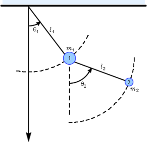
Figure 1. Coupled Pendulum.
Problem Statement
Consider the double-pendulum system consisting of a pendulum attached to another pendulum shown in Figure 1.
Assumptions:
- the system oscillates vertically under the influence of gravity.
- the mass of both rod are neligible
- no dumpung forces act on the system
- positive direction to the right.
The system of differential equations describing the motion is nonlinear


In order to linearize these equations, we assume that the displacements  and
and  are small enough so that
  and
and  . Thus,


Solution
Since our concern is about the motion functions, we will assign the masses  and
and  , the rod lenghts
  and
and  , and gravitational force
  constants to different variables as follows,

Hence,


Solving for  and
and  we obtain,


Therefore,


State Space

Let's plug some numbers. Knowing  , and assuming that
  ,
,  , and
, and  , the constants defined previously become,

Hence, the state space matrix is,

Eigenvalues
The eigenvalues are obtained from  's identity matrix,
![{\displaystyle [\lambda I-A]={\begin{bmatrix}\lambda &1&0&0\\-{\dfrac {8}{3}}&\lambda &{\dfrac {2}{3}}&0\\0&0&\lambda &1\\{\dfrac {8}{3}}&0&-{\dfrac {8}{3}}&\lambda \\\end{bmatrix}}}](https://wikimedia.org/api/rest_v1/media/math/render/svg/e5690dbcedd350d2117d03353097c9442e8eef25)
According to my TI-89, the eigenvalues are,


and the eigenvectors,

Standard Equation
Now, we plug the eigenvalues and eigenvectors to produce the standar equation,


= Matrix Exponential
Now we can use the equation for a transfer function to help us solve through the use of matrix exponentials.

This can be rearranged by multiplying T-inverse to the left side of the equations.

Now we can bring in the standard form of a state space equation

Combining the two equations we then get


![{\displaystyle [\lambda I-A]={\begin{bmatrix}\lambda &1&0&0\\-{\dfrac {8}{3}}&\lambda &{\dfrac {2}{3}}&0\\0&0&\lambda &1\\{\dfrac {8}{3}}&0&-{\dfrac {8}{3}}&\lambda \\\end{bmatrix}}}](https://wikimedia.org/api/rest_v1/media/math/render/svg/e5690dbcedd350d2117d03353097c9442e8eef25)


