HW 3: Difference between revisions
Jump to navigation
Jump to search
Created page with 'Doing this assignment taught many new lessons, in both sampling and octave.' |
No edit summary |
||
| (5 intermediate revisions by the same user not shown) | |||
| Line 1: | Line 1: | ||
Doing this assignment taught many new lessons, in both sampling and | Doing this assignment taught many new lessons, in both sampling and Octave. | ||
An infinite integral in Octave would be impractical. As a result, I did the following: | |||
* I made a vector "x" from -5 to 5 with points spaced every .02 in between. I originally made the vector from -10 to 10 with an even smaller spacing ([http://en.wikipedia.org/wiki/Nyquist%E2%80%93Shannon_sampling_theorem the Nyquist theorem] requires that samples must be taken at at least twice the frequency), but the integral took too long. | |||
* I made a vector "y" equal to "x". | |||
* I used the meshgrid function in Octave to make my vectors square matrices xx and yy ([http://www.network-theory.co.uk/docs/octave3/octave_159.html more info here]) | |||
* I then integrated <math>\ e^{(j2\pi*xx*yy)}</math> and plotted the result. | |||
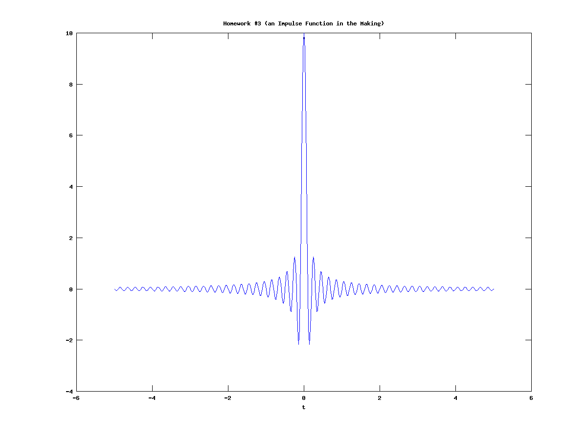
As you can see by the graph below, it is indeed very similar to an impulse function. To confirm, I integrated under the plot and found the area to be 0.99621, which is very close to the expected value of 1. | |||
[[File:HW3.png]] | |||
===Author=== | |||
[[Christopher Garrison Lau I]] | |||
Latest revision as of 21:18, 13 October 2010
Doing this assignment taught many new lessons, in both sampling and Octave. An infinite integral in Octave would be impractical. As a result, I did the following:
- I made a vector "x" from -5 to 5 with points spaced every .02 in between. I originally made the vector from -10 to 10 with an even smaller spacing (the Nyquist theorem requires that samples must be taken at at least twice the frequency), but the integral took too long.
- I made a vector "y" equal to "x".
- I used the meshgrid function in Octave to make my vectors square matrices xx and yy (more info here)
- I then integrated and plotted the result.
As you can see by the graph below, it is indeed very similar to an impulse function. To confirm, I integrated under the plot and found the area to be 0.99621, which is very close to the expected value of 1.
