Mark's Homework 15: Difference between revisions
| (4 intermediate revisions by the same user not shown) | |||
| Line 3: | Line 3: | ||
==MATLAB Script== | ==MATLAB Script== | ||
<pre> | <pre> | ||
%Author: Mark Priddy | |||
%Homework #15 MATLAB script | |||
%Description: Demonstrates oversampling and cancelling of the effects of the D/A converter | |||
clear all; | clear all; | ||
close all; | close all; | ||
%Number of sample points for our original signal | |||
N = 20; | |||
T=tmax/N; | %Time, in seconds, to extend our original signal. We then sample this signal N times | ||
t=0:T:(N)*T; | tmax=2; | ||
x=sin(2*pi*t)+sin(2*pi*2*t)+sin(2*pi*5*t); % | %Number of oversampling points | ||
oversampling = 4; | |||
%Calculations | |||
T=tmax/N; | |||
t=0:T:(N-1)*T; | |||
%This is our signal to over sample | |||
x=sin(2*pi*t)+sin(2*pi*2*t)+sin(2*pi*5*t); | |||
%The following three lines is our oversampling/interpolating filter | |||
N1=(oversampling-1)*N; | N1=(oversampling-1)*N; | ||
X=fft(x); | X=fft(x); | ||
X1 = (N1+N)/N*[X(1:N/2), zeros(1, N1), X(N/2+1:N)]; | X1 = (N1+N)/N*[X(1:N/2), zeros(1, N1), X(N/2+1:N)]; | ||
%This preserves our interpolated signal for graphing later on | |||
x2= ifft(X1); | x2= ifft(X1); | ||
% | |||
%This is to cancel out the effects of the D/A Converter | %This is to cancel out the effects of the D/A Converter | ||
% | |||
%sT is how many times we are going to sample our pulse p(t) | |||
sT = T*oversampling; | |||
%This is how wide our pulse has to be when we oversample | |||
stmax = oversampling*T; | |||
%This is the total number of sampling points for sampling p(t) | |||
sN = stmax/sT; | |||
t = 0:sT:stmax-sT; | t = 0:sT:stmax-sT; | ||
p = u(t+1e-9) - u(t-T/(2*oversampling)) + u(t - (oversampling*T-T/(2*oversampling))); % | %This is p(t), the pulse of the D/A converter, sampled at our oversampling rate | ||
p = u(t+1e-9) - u(t-T/(2*oversampling)) + u(t - (oversampling*T-T/(2*oversampling))); | |||
%P(f) is calculated: | |||
P = fft(p); | P = fft(p); | ||
% | %Take 1/P(f) so we cancel the effects of the D/A converter (which is P(f)) | ||
iP = 1./P; | |||
%Element multiply our interpolating filter with our D/A converter effect canceller filter | |||
X1 = X1 .* iP; | |||
x1 = ifft(X1); | x1 = ifft(X1); | ||
%Figure 1 plots the original signal and our interpolated signal (with D/A | % | ||
%Graphs | |||
% | |||
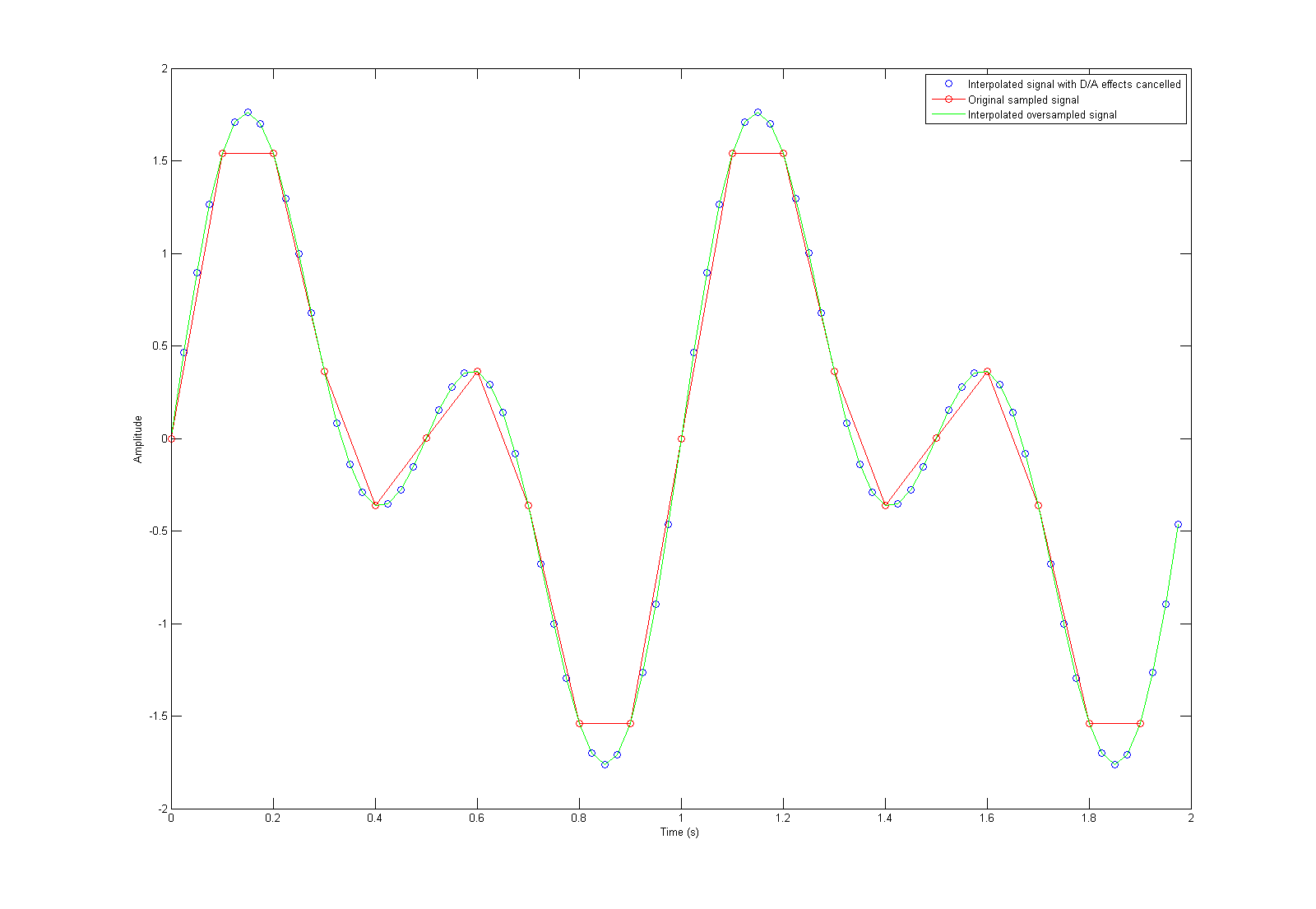
%Figure 1 plots the original signal and our interpolated signal (with D/A converter effects cancelled.) | |||
figure(1) | figure(1) | ||
t1 = 0:N/(N+N1)*T:(N-1/(N1+N))*T; | t1 = 0:N/(N+N1)*T:(N-1/(N1+N))*T; | ||
t=0:T:(N-1)*T; | |||
plot(t1, x1, 'bo', t, x, 'r-o', t1, x2, 'g-'); | |||
t=0:T:(N)*T; | legend('Interpolated signal with D/A effects cancelled', 'Original sampled signal', 'Interpolated oversampled signal') | ||
plot( | xlabel('Time (s)'); | ||
ylabel('Amplitude'); | |||
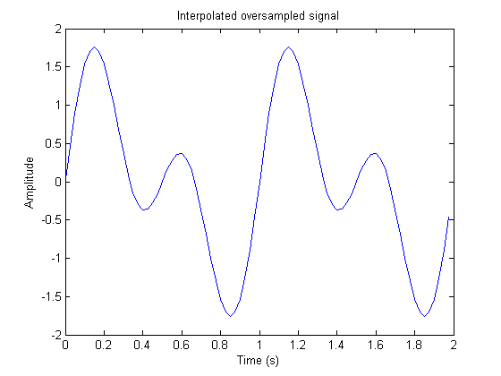
%Figure 2 plots just our interpolated signal, but this time with lines | %Figure 2 plots just our interpolated signal, but this time with lines connecting each point. | ||
figure(2) | figure(2) | ||
plot(t1, x1, 'b-'); | plot(t1, x1, 'b-'); | ||
title('Interpolated oversampled signal'); | |||
xlabel('Time (s)'); | |||
ylabel('Amplitude'); | |||
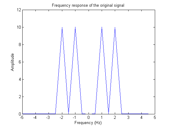
%Figure 3 plots the frequency response of our original sampled signal. | %Figure 3 plots the frequency response of our original sampled signal. | ||
figure(3) | figure(3) | ||
f = -1/(2*T):1/(N*T):1/(2*T)-1/(N*T); | f = -1/(2*T):1/(N*T):1/(2*T)-1/(N*T); | ||
plot(f,abs( | plot(f,abs(fftshift(X))) | ||
title('Frequency response of the original signal'); | |||
xlabel('Frequency (Hz)'); | |||
ylabel('Amplitude'); | |||
</pre> | </pre> | ||
To run this script, you'll also need another script, called "u.m" with the following contained inside. This must be located in the same folder as the main script above. | |||
<pre> | |||
function [out] = u(t) | |||
out=(1+sign(t))./2; | |||
end | |||
</pre> | |||
I couldn't find MATLAB's step function, so I created my own. | |||
==Graphs== | ==Graphs== | ||
[[Image:OVR20071203Fig1.png|thumb|left|1600px| Figure 1. The signals.]] | |||
[[Image:OVR20071203Fig2.png|thumb|left|694px| Figure 2. The interpolated signal.]] | |||
[[Image:OVR20071203Fig3.png|thumb|left|894px| Figure 3. The frequency response of the original signal.]] | |||
<br clear="all"/> | |||
==Explanations== | ==Explanations== | ||
Actually, this homework was relatively straight-forward. I sampled a signal, and ran it through the interpolation filter. The filter works by inserting (oversampling rate) - 1 times the number of points on the original DFT of the sampled signal. This causes the signal to be interpolated as well as oversampled. | |||
For canceling out the effects of the D/A converter, I simply DFT'd the pulse that a D/A converter would output, inverted it, and multiplied it with the DFT of my interpolating filter. This cancels out the effects of the D/A converter. There is hardly a difference due to oversampling. When you oversample the signal, the D/A converter pulse becomes much wider, so the edges where it goes down to zero don't go down to zero anymore. If that made any sense... | |||
Latest revision as of 18:07, 3 December 2007
Problem
Make a MATLAB script to do four times oversampling and a filter so as to eliminate as much as possible the effect of the D/A converter that follows the interpolation filter.
MATLAB Script
%Author: Mark Priddy
%Homework #15 MATLAB script
%Description: Demonstrates oversampling and cancelling of the effects of the D/A converter
clear all;
close all;

%Number of sample points for our original signal
N = 20;
%Time, in seconds, to extend our original signal. We then sample this signal N times
tmax=2;
%Number of oversampling points
oversampling = 4;

%Calculations
T=tmax/N;
t=0:T:(N-1)*T;

%This is our signal to over sample
x=sin(2*pi*t)+sin(2*pi*2*t)+sin(2*pi*5*t);

%The following three lines is our oversampling/interpolating filter
N1=(oversampling-1)*N;
X=fft(x);
X1 = (N1+N)/N*[X(1:N/2), zeros(1, N1), X(N/2+1:N)];

%This preserves our interpolated signal for graphing later on
x2= ifft(X1);

%
%This is to cancel out the effects of the D/A Converter
%
%sT is how many times we are going to sample our pulse p(t)
sT = T*oversampling;
%This is how wide our pulse has to be when we oversample
stmax = oversampling*T;
%This is the total number of sampling points for sampling p(t)
sN = stmax/sT;
t = 0:sT:stmax-sT;
%This is p(t), the pulse of the D/A converter, sampled at our oversampling rate
p = u(t+1e-9) - u(t-T/(2*oversampling)) + u(t - (oversampling*T-T/(2*oversampling)));
%P(f) is calculated:
P = fft(p);

%Take 1/P(f) so we cancel the effects of the D/A converter (which is P(f))
iP = 1./P;

%Element multiply our interpolating filter with our D/A converter effect canceller filter
X1 = X1 .* iP;
x1 = ifft(X1);

%
%Graphs
%
%Figure 1 plots the original signal and our interpolated signal (with D/A converter effects cancelled.)
figure(1)
t1 = 0:N/(N+N1)*T:(N-1/(N1+N))*T;
t=0:T:(N-1)*T;
plot(t1, x1, 'bo', t, x, 'r-o', t1, x2, 'g-');
legend('Interpolated signal with D/A effects cancelled', 'Original sampled signal', 'Interpolated oversampled signal')
xlabel('Time (s)');
ylabel('Amplitude');

%Figure 2 plots just our interpolated signal, but this time with lines connecting each point.
figure(2)
plot(t1, x1, 'b-');
title('Interpolated oversampled signal');
xlabel('Time (s)');
ylabel('Amplitude');

%Figure 3 plots the frequency response of our original sampled signal.
figure(3)
f = -1/(2*T):1/(N*T):1/(2*T)-1/(N*T);
plot(f,abs(fftshift(X)))
title('Frequency response of the original signal');
xlabel('Frequency (Hz)');
ylabel('Amplitude');
To run this script, you'll also need another script, called "u.m" with the following contained inside. This must be located in the same folder as the main script above.
function [out] = u(t)
out=(1+sign(t))./2;
end
I couldn't find MATLAB's step function, so I created my own.
Graphs


Explanations
Actually, this homework was relatively straight-forward. I sampled a signal, and ran it through the interpolation filter. The filter works by inserting (oversampling rate) - 1 times the number of points on the original DFT of the sampled signal. This causes the signal to be interpolated as well as oversampled.
For canceling out the effects of the D/A converter, I simply DFT'd the pulse that a D/A converter would output, inverted it, and multiplied it with the DFT of my interpolating filter. This cancels out the effects of the D/A converter. There is hardly a difference due to oversampling. When you oversample the signal, the D/A converter pulse becomes much wider, so the edges where it goes down to zero don't go down to zero anymore. If that made any sense...