Laplace transforms: Critically Damped Spring Mass system: Difference between revisions
Jump to navigation
Jump to search
No edit summary |
|||
| (12 intermediate revisions by the same user not shown) | |||
| Line 13: | Line 13: | ||
<math>m=\frac{98}{9.81}</math> | <math>m=\frac{98}{9.81}kg</math> | ||
<math>\text {Spring Constant k=40}\,</math> | <math>\text {Spring Constant k=40}N/m\,</math> | ||
<math>\text {Damping Constant C=40}\,</math> | <math>\text {Damping Constant C=40}\,</math> | ||
| Line 82: | Line 82: | ||
<math>\text {So as you can see the value for the initial position will be 0. Because the infinity in the denominator always makes the function tend toward zero.}\,</math> | <math>\text {So as you can see the value for the initial position will be 0.}\,</math> | ||
<math>\text {Because the infinity in the denominator always makes the function tend toward zero.}\,</math> | |||
<math>\text {Which makes sense because the system is initially in equilibrium. }\,</math> | <math>\text {Which makes sense because the system is initially in equilibrium. }\,</math> | ||
| Line 94: | Line 95: | ||
<math>\text {This shows the final value to be}\,</math> | <math>\text {This shows the final value to be}\,</math> | ||
<math>-\frac{4}{4} | <math>-\frac{4}{4}m</math> | ||
<math>\text {Which appears to mean the system will be right below equilibrium after a long time. }\,</math> | <math>\text {Which appears to mean the system will be right below equilibrium after a long time. }\,</math> | ||
| Line 116: | Line 117: | ||
==Break Points== | ==Break Points== | ||
Find the Break points using the transfer function | <math>\text {Find the Break points using the transfer function.}\,</math> | ||
==Transfer fucntion== | ===Transfer fucntion=== | ||
<math>\mathbf {X}(s)=-\frac{4}{(s+2)^2} </math><br /><br /> | <math>\mathbf {X}(s)=-\frac{4}{(s+2)^2} </math><br /><br /> | ||
<math>\text {The equation above contains break points but only in the denominator.}\,</math> | |||
<math>\text {There is only the variable s in the denominator so only those types of break point exist}\,</math> | |||
<math>\text {The break points are asymtotes at the point -2 which occurs twice in this particular equation}\,</math> | |||
==Convolution== | |||
<math>\text {The convolution equation is as follows: }\,</math> | |||
<math> | |||
x(t)=x_{in}(t) * h(t) = \int_{0}^{t} {x(t_0) \, h(t-t_0) \, dt_0} | |||
</math> | |||
<math>\text {It does basically the same thing as the Laplace Transform. }\,</math> | |||
<math>\text {To start we must inverse transform our transfer function }\,</math> | |||
<math>\mathbf {X}(s)=-\frac{4}{(s+2)^2} </math><br /><br /> | |||
<math>\text {Which once more yields: }\,</math> | |||
<math>\mathbf {x}(t)=-4te^{-2t}</math><br /><br /> | |||
<math>\text {Then we put this into the convolution integral: }\,</math> | |||
<math> | |||
x(t)=x_{in}(t) * h(t) = \int_{0}^{t} {-4(t-t_0)e^{-2t-t_0} \, dt_0} | |||
</math> | |||
<math>\text {Which once more yeilds: }\,</math> | |||
<math>\mathbf {x}(t)=(-cte^{-2t})</math><br /><br /> | |||
<math>\text {Not exactly the same but remember initial conditions arnt used}\,</math> | |||
==State Space== | |||
<math>\text {Using state equatons is just another way to solve a system modeled by an ODE }\,</math> | |||
<math>\text {First we need to add an applied force so u(t)=2N }\,</math> | |||
<math>m=\frac{98.1}{9.81}=10 kg</math> | |||
<math>\text {k=40}\,</math> | |||
<math>\text {C=40}\,</math> | |||
<math>\text {x(0)=0}\,</math> | |||
<math>\dot{x}(0)=-4</math> | |||
<math>\ddot{x}(0)=0</math> | |||
<math>\begin{bmatrix} \dot{x} \\ \ddot{x} \end{bmatrix}=\begin{bmatrix} 0 & 1 \\ -k/m & -C/m \end{bmatrix} \begin{bmatrix} x \\ \dot{x} \end{bmatrix} + \begin{bmatrix} 0 \\ 1/m \end{bmatrix}u(t)</math> | |||
Created by Greg Peterson | Created by Greg Peterson | ||
Checked by Mark Bernet | Checked by Mark Bernet | ||
Latest revision as of 14:26, 10 December 2009
Using the Laplace Transform to solve a spring mass system that is critically damped
Problem Statement
An 98 Newton weight is attached to a spring with a spring constant k of 40 N/m. The spring is stretched 4 m and rests at its equilibrium position. It is then released from rest with an initial upward velocity of 2 m/s. The system contains a damping force of 40 times the initial velocity.
Solution
Given
Solving the problem
Apply the Initial and Final Value Theorems to find the initial and final values
- Initial Value Theorem
- Final Value Theorem
Applying this to our problem
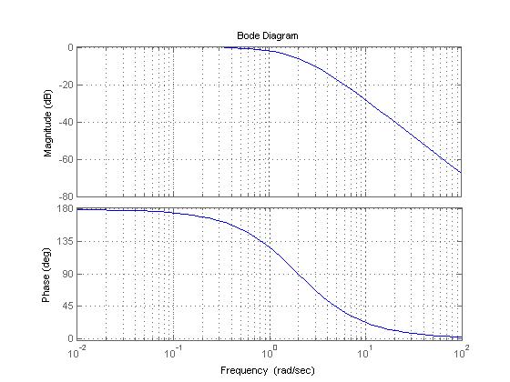
Bode Plot of the transfer function
Transfer Function
Bode Plot

Break Points
Transfer fucntion
Convolution
State Space
Created by Greg Peterson
Checked by Mark Bernet