Quadrature sampling waveform plot - HW10

Max Woesner

Back to my Home Page

Homework #10 - Quadrature sampling waveform plot

Problem Statement

Plot $\ {\frac {2}{T}}\sum _{n=1}^{\infty }sin{\bigg (}{\frac {2\pi nt}{T}}{\bigg )}\!$

Solution

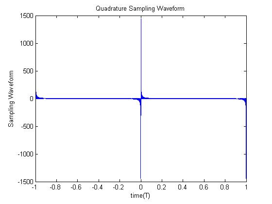
While we can't sum to infinity in the computer, we can get a close approximation summing over a large enough range of $n\!$

I found summing over $n=1:1000\!$ was about the most the computer could handle reasonably.

The following script was written in MATLAB to produce the desired plot.

clear all;
close all;
sum = 0;
T = 1;
t = -T:0.0001:T;
N = 1000;
for n = 1:N;
     if n==0
          h = 0;
     else
          h = 2/T;
     end
     sum = sum+h*sin(2*pi*n*t/T);
end
plot(t,sum)
title('Quadrature Sampling Waveform')
xlabel('time(T)')
ylabel('Sampling Waveform')

Running the MATLAB script above gives us the following plot.

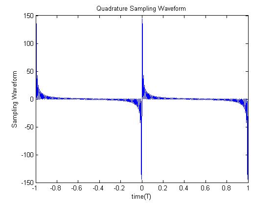
Summing over a smaller range of $n\!$ would look like the following.

clear all;
close all;
sum = 0;
T = 1;
t = -T:0.001:T;
N = 100;
for n = 1:N;
     if n==0
          h = 0;
     else
          h = 2/T;
     end
     sum = sum+h*sin(2*pi*n*t/T);
end
plot(t,sum)
title('Quadrature Sampling Waveform')
xlabel('time(T)')
ylabel('Sampling Waveform')