Coupled Oscillator: Hellie: Difference between revisions

Latest revision as of 23:28, 13 December 2009

Problem Statement

Write up on the Wiki a solution of a coupled oscillator problem like the coupled pendulum. Use State Space methods. Describe the eigenmodes of the system. Solve Using the Matrix Exponential

Initial Conditions:

m_{1} = 10 k g

m_{2} = 10 k g

k 1 = 100 N / m

k 2 = 150 N / m

k 3 = 100 N / m

F=ma

\ddot{x_{1}} = \frac{x_{1} (k_{1} - k_{2})}{m_{1}} - \frac{x_{2} * k_{1}}{m_{1}}

\ddot{x_{2}} = \frac{x_{2} (k_{1} + k_{2})}{m_{2}} - \frac{x_{1} * k_{1}}{m_{2}}

State Equations

$[\begin{matrix} \dot{x_{1}} \\ \ddot{x_{1}} \\ \dot{x_{2}} \\ \ddot{x_{2}} \end{matrix}]$ = $[\begin{matrix} 0 & 1 & 0 & 0 \\ \frac{(k_{1} - k_{2})}{m_{1}} & 0 & \frac{- k_{1}}{m_{1}} & 0 \\ 0 & 0 & 0 & 1 \\ \frac{- k_{1}}{m_{2}} & 0 & \frac{(k_{1} + k_{2})}{m_{2}} & 0 \end{matrix}] [\begin{matrix} x_{1} \\ {\dot{x}}_{1} \\ x_{2} \\ {\dot{x}}_{2} \end{matrix}] + [\begin{matrix} 0 & 0 & 0 & 0 \\ 0 & 0 & 0 & 0 \\ 0 & 0 & 0 & 0 \\ 0 & 0 & 0 & 0 \end{matrix}] [\begin{matrix} 0 \\ 0 \\ 0 \\ 0 \end{matrix}]$

With the numbers...

$[\begin{matrix} \dot{x_{1}} \\ \ddot{x_{1}} \\ \dot{x_{2}} \\ \ddot{x_{2}} \end{matrix}]$ = $[\begin{matrix} 0 & 1 & 0 & 0 \\ \frac{(- 50 N / m)}{10 k g} & 0 & \frac{- 100 N / m}{10 k g} & 0 \\ 0 & 0 & 0 & 1 \\ \frac{- 100 N / m}{10 k g} & 0 & \frac{(250 N / m)}{10 k g} & 0 \end{matrix}] [\begin{matrix} x_{1} \\ {\dot{x}}_{1} \\ x_{2} \\ {\dot{x}}_{2} \end{matrix}]$

$[\begin{matrix} \dot{x_{1}} \\ \ddot{x_{1}} \\ \dot{x_{2}} \\ \ddot{x_{2}} \end{matrix}]$ = $[\begin{matrix} 0 & 1 & 0 & 0 \\ - 5 & 0 & - 10 & 0 \\ 0 & 0 & 0 & 1 \\ - 10 & 0 & 25 & 0 \end{matrix}] [\begin{matrix} x_{1} \\ {\dot{x}}_{1} \\ x_{2} \\ {\dot{x}}_{2} \end{matrix}]$

Eigenvalues

λ_{1} = - 5.29412

λ_{2} = 2.83333 i

λ_{3} = - 2.83333 i

λ_{4} = 0

Eigenvectors

k_{1} = [\begin{matrix} - . 05379 \\ . 28475 \\ . 17764 \\ - . 94046 \end{matrix}]

k_{2} = [\begin{matrix} - . 31854 i \\ . 90253 \\ - . 09645 i \\ . 27326 \end{matrix}]

k_{3} = [\begin{matrix} . 31854 i \\ . 90253 \\ . 09645 i \\ . 27326 \end{matrix}]

k_{4} = [\begin{matrix} - . 05379 \\ - . 28475 \\ . 17764 \\ . 94046 \end{matrix}]

Standard Equation

x = c_{1} k_{1} e^{λ_{1} t} + c_{2} k_{2} e^{λ_{2} t} + c_{3} k_{3} e^{λ_{3} t} + c_{4} k_{4} e^{λ_{4} t}

x = c_{1}

[\begin{matrix} - . 05379 \\ . 28475 \\ . 17764 \\ - . 94046 \end{matrix}]

e^{- 5.29412} + c_{2}

[\begin{matrix} - . 31854 i \\ . 90253 \\ - . 09645 i \\ . 27326 \end{matrix}]

e^{2.83333 i} + c_{3}

[\begin{matrix} . 31854 i \\ . 90253 \\ . 09645 i \\ . 27326 \end{matrix}]

e^{- 2.83333 i} + c_{4}

[\begin{matrix} - . 05379 \\ - . 28475 \\ . 17764 \\ . 94046 \end{matrix}]

e^{0}

Eigenmodes

There are two eigenmodes for the system

1) m1 and m2 oscillating together

2) m1 and m2 oscillating at exactly a half period difference

Matrix Exponential using transformation z=Tx

$T^{- 1} = [k_{1} | k_{2} | k_{3} | k_{4}]$

$z = T x$

$\dot{z} = T A T^{- 1} z$

$\dot{z} =$ $[\begin{matrix} - 5.2941 & 0 & 0 & 0 \\ 0 & 2.833 i & 0 & 0 \\ 0 & 0 & - 2.83333 i & 0 \\ 0 & 0 & 0 & 5.2941 \end{matrix}]$ $z$

$B = T A T^{- 1} = [\begin{matrix} - 5.2941 & 0 & 0 & 0 \\ 0 & 2.833 i & 0 & 0 \\ 0 & 0 & - 2.83333 i & 0 \\ 0 & 0 & 0 & 5.2941 \end{matrix}]$

$z = e^{B t} z (0)$

$e^{B t} = [\begin{matrix} e^{- 5.2941 t} & 0 & 0 & 0 \\ 0 & e^{2.833 i t} & 0 & 0 \\ 0 & 0 & e^{- 2.83333 i t} & 0 \\ 0 & 0 & 0 & e^{5.2941 t} \end{matrix}]$

$x = T^{- 1} z$

$x = T^{- 1} e^{B t} T x (0)$

$e^{P t} = T^{- 1} e^{B t} T$

$e^{P t} =$ lots of variables

Another way to solve using the Matrix exponential

$e^{A t} = ℒ^{- 1} {[S I - A]^{- 1}}$

$[S I - A]$ = $[\begin{matrix} S & 1 & 0 & 0 \\ \frac{(- 50 N / m)}{15 k g} & S & \frac{- 100 N / m}{15 k g} & 0 \\ 0 & 0 & S & 1 \\ \frac{100 N / m}{15 k g} & 0 & \frac{(250 N / m)}{15 k g} & S \end{matrix}]$

$[S I - A]^{- 1} =$ (something too large for my calculator to display or that I want to type out)

$ℒ^{- 1} {[S I - A]^{- 1}} =$ (something too large for my calculator to display or that I want to type out)

Written by: Andrew Hellie

@@ Line 1: / Line 1: @@
 ===Problem Statement===
-'''Write up on the Wiki a solution of a coupled oscillator problem like the coupled pendulum.  Use State Space methods.  Describe the eigenmodes of the system.'''
+'''Write up on the Wiki a solution of a coupled oscillator problem like the coupled pendulum.  Use State Space methods.  Describe the eigenmodes of the system.  Solve Using the Matrix Exponential'''
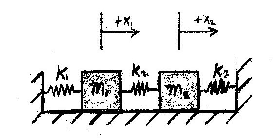
    [[Image:Coupled_Oscillator.jpg]]
 '''Initial Conditions:'''
-:<math>m_1= 15 kg\,</math>
+:<math>m_1= 10 kg\,</math>
-:<math>m_2 = 15 kg\,</math>
+:<math>m_2 = 10 kg\,</math>
 :<math>k1=100 N/m\,</math>
@@ Line 15: / Line 16: @@
 :<math>k3=100 N/m\,</math>
+'''F=ma'''
+:<math>\ddot{x_1}=\frac{x_1(k_1-k_2)}{m_1}-\frac{x_2*k_1}{m_1}\,</math>
+:<math>\ddot{x_2}=\frac{x_2(k_1+k_2)}{m_2}-\frac{x_1*k_1}{m_2}\,</math>
 '''State Equations'''
@@ Line 32: / Line 37: @@
 \frac{(k_1-k_2)}{m_1}&0&\frac{-k_1}{m_1}&0 \\
 &0&0&1 \\
-\frac{k_1}{m_2}&0&\frac{(k_1+k_2)}{m_2}&0
+\frac{-k_1}{m_2}&0&\frac{(k_1+k_2)}{m_2}&0
 \end{bmatrix}
@@ Line 75: / Line 80: @@
 \begin{bmatrix}
 &1&0&0 \\
-\frac{(-50 N/m)}{15 kg}&0&\frac{-100 N/m}{15 kg}&0 \\
+\frac{(-50 N/m)}{10 kg}&0&\frac{-100 N/m}{10 kg}&0 \\
 &0&0&1 \\
-\frac{100 N/m}{15 kg}&0&\frac{(250 N/m)}{15 kg}&0
+\frac{-100 N/m}{10 kg}&0&\frac{(250 N/m)}{10 kg}&0
 \end{bmatrix}
@@ Line 90: / Line 95: @@
 </math>
+<math>
+\begin{bmatrix}
+\dot{x_1} \\
+\ddot{x_1} \\
+\dot{x_2} \\
+\ddot{x_2}
+\end{bmatrix}\,
+</math>
+=
+<math>
+\begin{bmatrix}
+&1&0&0 \\
+-5&0&-10&0 \\
+&0&0&1 \\
+-10&0&25&0
+\end{bmatrix}
+\begin{bmatrix}
+x_1 \\
+\dot{x}_1 \\
+x_2 \\
+\dot{x}_2
+\end{bmatrix}
+</math>
+'''Eigenvalues'''
+:<math>\lambda_1=-5.29412\,</math>
+:<math>\lambda_2=2.83333i\,</math>
+:<math>\lambda_3= -2.83333i\,</math>
+:<math>\lambda_4=0\,</math>
+'''Eigenvectors'''
+:<math>k_1=\begin{bmatrix}
+-.05379\\
+.28475 \\
+.17764 \\
+-.94046
+\end{bmatrix}</math>
+:<math>k_2=\begin{bmatrix}
+-.31854i\\
+.90253 \\
+-.09645i\\
+.27326
+\end{bmatrix}</math>
+:<math>k_3=\begin{bmatrix}
+.31854i\\
+.90253 \\
+.09645i \\
+.27326
+\end{bmatrix}</math>
+:<math>k_4=\begin{bmatrix}
+-.05379\\
+-.28475 \\
+.17764 \\
+.94046
+\end{bmatrix}</math>
+'''Standard Equation'''
+:<math>x=c_1k_1e^{\lambda_1 t}+c_2k_2e^{\lambda_2 t}+c_3k_3e^{\lambda_3 t}+c_4k_4e^{\lambda_4 t}</math>
+:<math>\ x=c_1</math><math>\begin{bmatrix}
+-.05379\\
+.28475 \\
+.17764 \\
+-.94046
+\end{bmatrix}\,</math><math>e^{-5.29412}+ c_2\,</math><math>
+\begin{bmatrix}
+-.31854i\\
+.90253 \\
+-.09645i\\
+.27326
+\end{bmatrix}\,</math><math>e^{2.83333i}+ c_3\,</math><math>\begin{bmatrix}
+.31854i\\
+.90253 \\
+.09645i \\
+.27326
+\end{bmatrix}\,</math><math>e^{-2.83333i}+ c_4\,</math><math>\begin{bmatrix}
+-.05379\\
+-.28475 \\
+.17764 \\
+.94046
+\end{bmatrix}\,
+</math><math>e^{0}\,</math>
 '''Eigenmodes'''
-:There are three eigenmodes for the system
+:There are two eigenmodes for the system
 ::1) m1 and m2 oscillating together
@@ Line 100: / Line 205: @@
+'''Matrix Exponential using transformation z=Tx'''
+<math>T^{-1}=[k_1|k_2|k_3|k_4]\,</math>
+<math>z=Tx\,</math>
+<math>\dot{z}=TAT^{-1}z \,</math>
+<math>\dot{z}=\,</math>
+<math>\begin{bmatrix}
+-5.2941&0&0&0 \\
+&2.833i&0&0 \\
+&0&-2.83333i&0 \\
+&0&0&5.2941
+\end{bmatrix}\,
+</math>
+<math>z\,</math>
+<math>B=TAT^{-1}=\begin{bmatrix}
+-5.2941&0&0&0 \\
+&2.833i&0&0 \\
+&0&-2.83333i&0 \\
+&0&0&5.2941
+\end{bmatrix}\,</math>
+<math>z=e^{Bt}z(0)\,</math>
+<math>e^{Bt}=\begin{bmatrix}
+e^{-5.2941t}&0&0&0 \\
+&e^{2.833it}&0&0 \\
+&0&e^{-2.83333it}&0 \\
+&0&0&e^{5.2941t}
+\end{bmatrix}\,</math>
+<math>x=T^{-1}z\,</math>
+<math>x=T^{-1}e^{Bt}Tx(0)\,</math>
+<math>e^{Pt}=T^{-1}e^{Bt}T\,</math>
+<math>e^{Pt}=\,</math>lots of variables
+'''Another way to solve using the Matrix exponential'''
+<math>e^{At}=\mathcal{L}^{-1}\left\{[SI-A]^{-1}\right\}\,</math>
+<math>[SI-A]\,</math>
+=
+<math>
+\begin{bmatrix}
+S&1&0&0 \\
+\frac{(-50 N/m)}{15 kg}&S&\frac{-100 N/m}{15 kg}&0 \\
+&0&S&1 \\
+\frac{100 N/m}{15 kg}&0&\frac{(250 N/m)}{15 kg}&S
+\end{bmatrix}
+</math>
-'''Solve Using the Matrix Exponential'''
+<math>[SI-A]^{-1} =\,</math> (something too large for my calculator to display or that I want to type out)
-<math>e^{At}=\mathcal{L}^{-1}\left\{(SI-A)^{-1}\right\},\,</math>
+<math>\mathcal{L}^{-1}\left\{[SI-A]^{-1}\right\} = \,</math>(something too large for my calculator to display or that I want to type out)
 Written by: Andrew Hellie

Coupled Oscillator: Hellie: Difference between revisions

Latest revision as of 23:28, 13 December 2009

Problem Statement

Navigation menu

Search