DFT Exploration by harrde: Difference between revisions
Jump to navigation
Jump to search
No edit summary |
|||
| Line 71: | Line 71: | ||
===Explanation=== | ===Explanation=== | ||
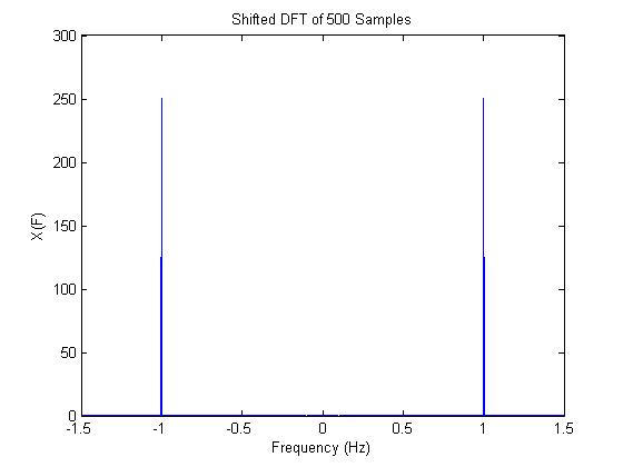
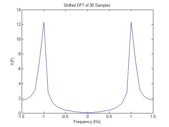
The DFT only gives us an approximation of the actual Fourier Transform, as was found in the last homework. With few sampling points the DFT hardly resembles the expected trasfrom. This is because the edge effects have a greater affect with fewer sample points. | The DFT only gives us an approximation of the actual Fourier Transform, as was found in the last homework. With few sampling points the DFT hardly resembles the expected trasfrom. This is because the edge effects have a greater affect with fewer sample points. | ||
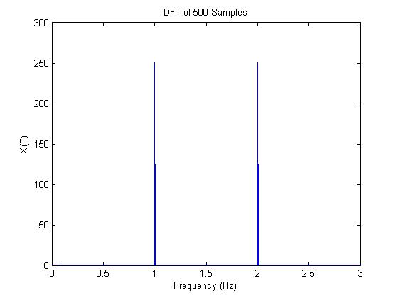
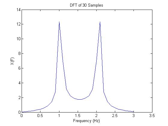
From the example above we see that the more sampling points we take the closer the DFT resembles the actual transform. e.g. with 30 sample points the DFT has "spikes" with height of about 12 but with 500 sample points they have a height of 250, which is obviously closer the expected Dirac delta funtions with infinite height. | |||
Latest revision as of 00:10, 7 December 2007
Problem Statement
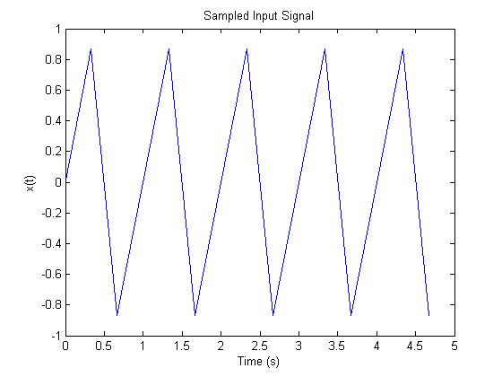
Sample at 3Hz, take the DFT, and explain the results.
Solution
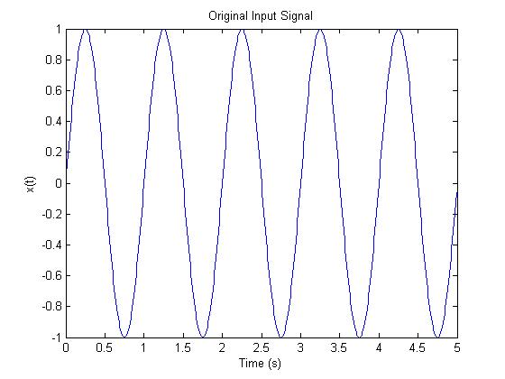
Here is the MATLAB code and resulting figures:
f = 3;              % Sampling freq.
T = 1/f;            % Sampling period
t = 0:.01:5;
N2 = 500;          % Number of sampling points
N3 = 30;
t2 = 0:T:N2*T;
t3 = 0:T:N3*T;

x = sin(2*pi*t);    % Signal that is sampled
x2 = sin(2*pi*t2);
x3 = sin(2*pi*t3);

X2 = fft(x2);         % DFT of long signal
X3 = fft(x3);         % DFT of short signal

figure(1)                    %Original signal
plot(t(1:500),x(1:500))
xlabel('Time (s)')
ylabel('x(t)')
title('Original Input Signal')

figure(2)
plot(t2(1:15),x2(1:15))      % Sampled signal
xlabel('Time (s)')
ylabel('x(t)')
title('Sampled Input Signal')

figure(3)                    %DFT of long signal
plot(t2/(N2*T*T),abs(X2))
xlabel('Frequency (s)')
ylabel('X(F)')
title('DFT of 500 Samples')

figure(4)                    % DFT of short signal
plot(t3/(N3*T*T),abs(X3))
xlabel('Frequency (s)')
ylabel('X(F)')
title('DFT of 30 Samples')

figure(5)                   % Shifted DFT of long signal
XS2=fftshift(X2);
f2=-1/(2*T):1/(N2*T):1/(2*T);
plot(f2,abs(XS2))
xlabel('Frequency (s)')
ylabel('X(F)')
title('Shifted DFT of 500 Samples')

figure(6)                   % Shifted DFT of short signal
XS3=fftshift(X3);
f3=-1/(2*T):1/(N3*T):1/(2*T);
plot(f3,abs(XS3))
xlabel('Frequency (s)')
ylabel('X(F)')
title('Shifted DFT of 30 Samples')
Explanation
The DFT only gives us an approximation of the actual Fourier Transform, as was found in the last homework. With few sampling points the DFT hardly resembles the expected trasfrom. This is because the edge effects have a greater affect with fewer sample points. From the example above we see that the more sampling points we take the closer the DFT resembles the actual transform. e.g. with 30 sample points the DFT has "spikes" with height of about 12 but with 500 sample points they have a height of 250, which is obviously closer the expected Dirac delta funtions with infinite height.
