Oversample and Predistort by harrde: Difference between revisions
No edit summary |
|||
| Line 76: | Line 76: | ||
===Explanation=== | ===Explanation=== | ||
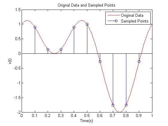
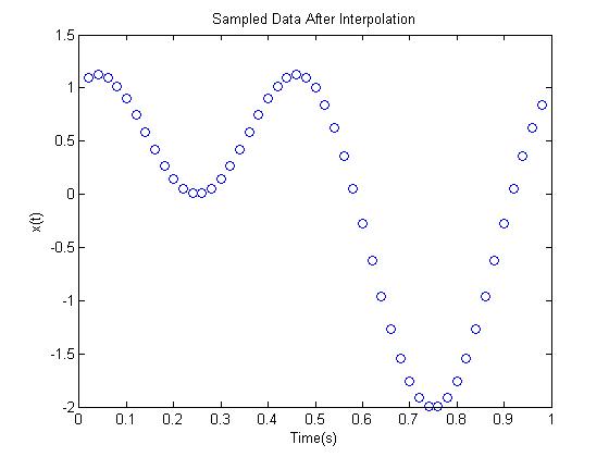
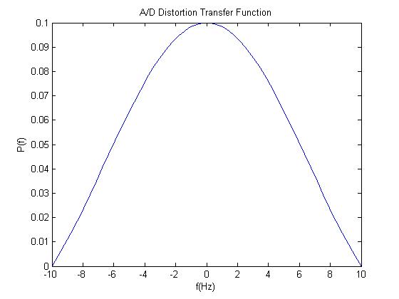
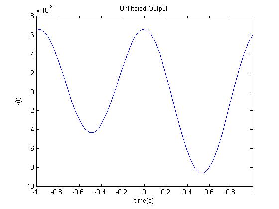
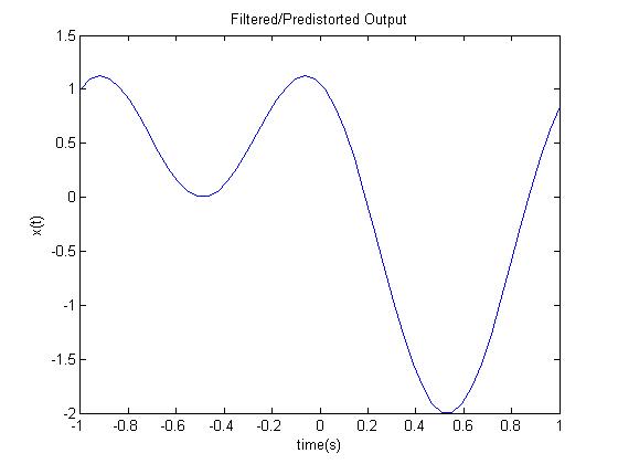
The five graphs show a signal at important times as it passes through this system; which is similar to a signal being stored on a CD and then played back. The first graph shows the original signal and the data gathered from sampling. The next graph shows the sampled data plus the interpolation points found through 4 times oversampling. The third graph is a depiction of the transfer function of the D/A converter. This transfer function distorts the output signal as seen in the fourth graph. This is why we pass the signal through a digital filter to predistort it so that at the output of our system it will not be distorted. The filter's transfer function is simply the reciprocal of the D/A converter's transfer function. | |||
Latest revision as of 16:07, 7 December 2007
Problem Statement
Make a MATLAB script to do four times oversampling and filter so as to eliminate as much as possible the effect of the D/A converter that follows the interpolating filter.
Solution
MATLAB script and results:
f = 10;             % Sampling freq.
T = 1/f;            % Sampling period
N = 10;             % Number of sampling points
t=0:T:(N-1)*T;
x=sin(2*pi*t)+cos(2*pi*2*t);   % Signal that is sampled
t_original = 0:.01:1;
x_original = sin(2*pi*t_original)+cos(2*pi*2*t_original);

OSample = 4;                            % How many times to oversampling

figure(1);
clf
plot(t_original,x_original,'r');         %Original signal sampled
hold on
stem(t,x)
xlabel('Time(s)');
ylabel('x(t)');
title('Orignal Data and Sampled Points')
hold
legend('Original Data','Sampled Points')

figure(2);
N1 = N*OSample;
X = fft(x);
X1 = (N1+N)/N*[X(1:N/2),zeros(1,N1),X(N/2+1:N)]; %This is the interpolation transfer function
x1 = ifft(X1);
t1=0:N/(N+N1)*T:(N-1/(N1+N))*T;
plot(t1,x1,'bo')                    %Sampled data with interpolation points
title('Sampled Data After Interpolation');
ylabel('x(t)');
xlabel('Time(s)');

%Now we will work on predistortion filter
f = linspace(-1/T,1/T,length(X1));
P = sin(pi*f*T)./(pi*f);                %Transfer function of A/D distortion
figure(3)
plot(f,P)                       % A/D distortion transfer function
title('A/D Distortion Transfer Function');
ylabel('P(f)');
xlabel('f(Hz)');

Out_unfiltered = X1.*P;
out_unfiltered = ifft(Out_unfiltered);

Out = X1.*(1./P).*P;
out = ifft(Out);

figure(4)
clf
plot(f./10,real(out_unfiltered))      %This is the output with out filter/predistortion
title('Unfiltered Output');
ylabel('x(t)');
xlabel('time(s)');

figure(5)
clf
plot(f./10,real(out))                 %This is the output with the filter
title('Filtered/Predistorted Output');
ylabel('x(t)');
xlabel('time(s)');
Explanation
The five graphs show a signal at important times as it passes through this system; which is similar to a signal being stored on a CD and then played back. The first graph shows the original signal and the data gathered from sampling. The next graph shows the sampled data plus the interpolation points found through 4 times oversampling. The third graph is a depiction of the transfer function of the D/A converter. This transfer function distorts the output signal as seen in the fourth graph. This is why we pass the signal through a digital filter to predistort it so that at the output of our system it will not be distorted. The filter's transfer function is simply the reciprocal of the D/A converter's transfer function.
