State Space Form: Difference between revisions
No edit summary |
No edit summary |
||
| Line 42: | Line 42: | ||
Or, more generally,<br> | Or, more generally,<br> | ||
<math>\mathbf{\dot x} = \mathbf{Ax+B}f</math><br> | <math>\mathbf{\dot x} = \mathbf{Ax+B}f</math><br> | ||
This is called the state space representation of the differential equation. | This is called the state space representation of the differential equation. This can be quite useful because the entire description of the differential equation is available in the matrix, and is easily manipulated using linear algebra. | ||
Example | -Example- | ||
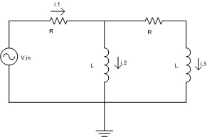
For the circuit below, find a set of state variable equations (there are several ways to do this, I will choose the one I feel is most intuitive.) | |||
[[Image:Circuit1.jpg]] | |||
Start by using loop (also known as mesh or KVL) analysis. | |||
Loop 1:<br> | |||
<math>-Vin +i_{1}*R + L*\frac{di_{2}}{dt}=0</math><br> | |||
Loop 2:<br> | |||
<math>-Vin +i_{1}*R + i_{3}*R + L*\frac{di_{3}}{dt} = 0</math><br> | |||
Lets let:<br> <math>x_{1}=i_{2}</math> and<br> <math> x_{2}=i_{3}</math><br> | |||
So, <math>i_{1}=x_{1}+x_{2}</math>. Substituting into the equations above, we get:<br> | |||
<math>-Vin +(x_{1}+x_{2})*R + L*\dot x_{1}=0</math> and<br> | |||
<math>-Vin +(x_{1}+x_{2})*R + x_{2}*R + L*\dot x_{2} = 0</math><br> | |||
Where <math>\dot x_{1}</math> is the derivative of <math>x</math>. | |||
Revision as of 12:03, 10 September 2010
In my Signals and Systems II class at University of Idaho, we are learning about the state space form of representing a solution to a LTI differential equation. I'll add more here soon.
Consider the differential equation
or
The state of this equation can be described using what is called state space form. State space form gives the blah blah more here.
let
let
so
We can now re-write the equation above to be:
so
and from the definition above
We can take this and put it into matrix form:
Or, more generally,
This is called the state space representation of the differential equation. This can be quite useful because the entire description of the differential equation is available in the matrix, and is easily manipulated using linear algebra.
-Example-
For the circuit below, find a set of state variable equations (there are several ways to do this, I will choose the one I feel is most intuitive.)

Start by using loop (also known as mesh or KVL) analysis.
Loop 1:
Loop 2:
Lets let:
and
So, . Substituting into the equations above, we get:
and
Where is the derivative of .