Chris' Page for HW 4 (Fourier Transforms)

The Fourier Transform is a process or formula that converts a signal from one domain to another. Often it is used to go between the time domain and the frequency domain.

Developed by Frenchman, Jean Baptiste Joseph Fourier (1768 - 1830), the Fourier Transform stems from the more general Fourier Analysis, which is the representation of a function with sine and cosine terms. Unlike the Fourier Series the Fourier Transform is capable of representing aperiodic signals.

Mathematical Description

The Fourier Transform is detonated by;

$$\begin{gathered} X(f)=\underset{-\mathrm{\infty }}{\overset{\mathrm{\infty }}{\int }}x(t) \\ {e}^{-j\omega t}dt, \end{gathered}$$

The Inverse Fourier Transform is;

$$\begin{gathered} x(t)=\frac{1}{2\pi }\underset{-\mathrm{\infty }}{\overset{\mathrm{\infty }}{\int }}X(\omega ) \\ {e}^{j\omega t}d\omega , \end{gathered}$$

Relation to Laplace Transform

Unless otherwise noted, a Laplace Transform is defined by the unilateral or one-sided integral

${ℒ}\{f(t)\}=\underset{0^{-}}{\overset{\mathrm{\infty }}{\int }}{e}^{-st}f(t)dt.$

The Laplace Transform can be applied from $-\mathrm{\infty }$ to $\mathrm{\infty }$, this is known as the Bilateral Laplace Transform and is denoted by

${ℒ}\{f(t)\}=\underset{-\mathrm{\infty }}{\overset{\mathrm{\infty }}{\int }}{e}^{-st}f(t)dt.$

Setting $s=j\omega$ ($\sigma =0$) gives the equation

${ℒ}\{f(t)\}=\underset{-\mathrm{\infty }}{\overset{\mathrm{\infty }}{\int }}{e}^{-j\omega t}f(t)dt.$

which is identical to the Fourier Transform. The same relationship exists between the Inverse Laplace and the Inverse Fourier transforms.

Examples

Below is a very basic example based on a Matlab help file.

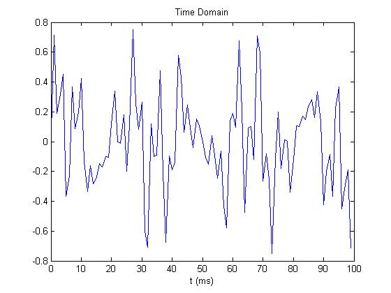
The time domain signal is produced by

t = 0:0.001:.1;

y = sin(2*pi*50*t)+sin(2*pi*120*t) +sin(2*pi*150*t) +sin(2*pi*310*t) +sin(2*pi*340*t);

y = 0.2 .* y;

The t matrix represents time vectors and y is the summation of sine functions of various frequencies, then y is redefined as 1/5 the original power.

Plotted with

figure(1)

plot(1000*t(1:100),y(1:100))

title('Time Domain')

xlabel('t (ms)')

yields

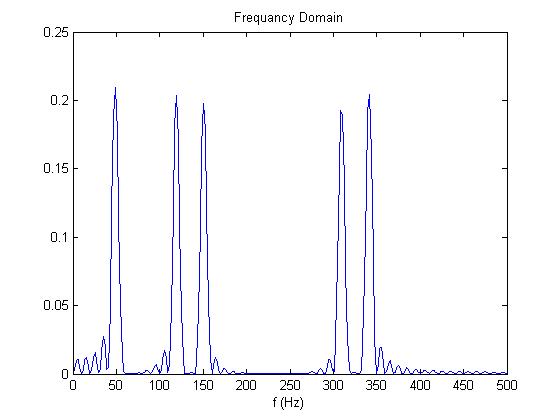
Then taking the Fourier Transform via the FFT and plotting

Y = fft(y,512);

Power = Y .* conj(Y) / 512;

f = 1000*(0:256)/512;

figure(2)

plot(f,Power(1:257))

title('Frequancy Domain')

xlabel('f (Hz)')

And if you want to hear it

wavwrite(y,1000,16,'test2.wav')

then

clear all

I believe that windowing needs to be added. Suggestions?