More about Sampling: Difference between revisions
Jump to navigation
Jump to search
No edit summary |
|||
| Line 9: | Line 9: | ||
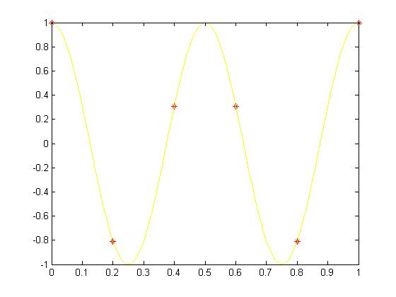
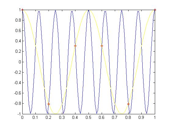
Like we can see in this images, the samples that we are getting out of the yellow wave, can be also samples in the blue one. | Like we can see in this images, the samples that we are getting out of the yellow wave, can be also samples in the blue one. | ||
Script for Matlab: | |||
clear all; | |||
t=0:.01:1; | |||
T=0.20; | |||
ts=0:T:1; | |||
f1=2; | |||
f2=1/0.125; | |||
plot(t,cos(2*pi*f2*t),'b-',ts,cos(2*pi*f1*ts),'r*',t,cos(2*pi*f1*t),'y-'); | |||
plot(ts,cos(2*pi*f1*ts),'r*',t,cos(2*pi*f1*t),'y-'); | |||
Revision as of 11:37, 12 November 2007
Aliasing
Aliasing is when different continuous signals become indistinguishable when sampled, this might happen when sampling too slow. It can also refer to the distortion that occurs when a signals are sampled and reconstructed as aliases of the original signals.
Here is an example of aliasing:
Like we can see in this images, the samples that we are getting out of the yellow wave, can be also samples in the blue one.
Script for Matlab:
clear all;
t=0:.01:1;
T=0.20;
ts=0:T:1;
f1=2;
f2=1/0.125;
plot(t,cos(2*pi*f2*t),'b-',ts,cos(2*pi*f1*ts),'r*',t,cos(2*pi*f1*t),'y-');
plot(ts,cos(2*pi*f1*ts),'r*',t,cos(2*pi*f1*t),'y-');

