Mark's Homework 15: Difference between revisions
Jump to navigation
Jump to search
No edit summary |
|||
| Line 3: | Line 3: | ||
==MATLAB Script== | ==MATLAB Script== | ||
<pre> | <pre> | ||
%Author: Mark Priddy | |||
%Homework #15 MATLAB script | |||
%Description: Demonstrates oversampling and cancelling of the effects of the D/A converter | |||
clear all; | clear all; | ||
close all; | close all; | ||
%Number of sample points for our original signal | |||
N = 20; | |||
T=tmax/N; | %Time, in seconds, to extend our original signal. We then sample this signal N times | ||
tmax=2; | |||
%Number of oversampling points | |||
oversampling = 4; | |||
%Calculations | |||
T=tmax/N; | |||
t=0:T:(N-1)*T; | t=0:T:(N-1)*T; | ||
x=sin(2*pi*t)+sin(2*pi*2*t)+sin(2*pi*5*t); % | |||
%This is our signal to over sample | |||
x=sin(2*pi*t)+sin(2*pi*2*t)+sin(2*pi*5*t); | |||
%The following three lines is our oversampling/interpolating filter | |||
N1=(oversampling-1)*N; | N1=(oversampling-1)*N; | ||
X=fft(x); | X=fft(x); | ||
X1 = (N1+N)/N*[X(1:N/2), zeros(1, N1), X(N/2+1:N)]; | X1 = (N1+N)/N*[X(1:N/2), zeros(1, N1), X(N/2+1:N)]; | ||
%This preserves our interpolated signal for graphing later on | |||
x2= ifft(X1); | x2= ifft(X1); | ||
% | |||
%This is to cancel out the effects of the D/A Converter | %This is to cancel out the effects of the D/A Converter | ||
% | |||
%sT is how many times we are going to sample our pulse p(t) | |||
sT = T*oversampling; | |||
%This is how wide our pulse has to be when we oversample | |||
stmax = oversampling*T; | |||
%This is the total number of sampling points for sampling p(t) | |||
sN = stmax/sT; | |||
t = 0:sT:stmax-sT; | t = 0:sT:stmax-sT; | ||
p = u(t+1e-9) - u(t-T/(2*oversampling)) + u(t - (oversampling*T-T/(2*oversampling))); % | %This is p(t), the pulse of the D/A converter, sampled at our oversampling rate | ||
p = u(t+1e-9) - u(t-T/(2*oversampling)) + u(t - (oversampling*T-T/(2*oversampling))); | |||
%P(f) is calculated: | |||
P = fft(p); | P = fft(p); | ||
% | %Take 1/P(f) so we cancel the effects of the D/A converter (which is P(f)) | ||
iP = 1./P; | |||
%Element multiply our interpolating filter with our D/A converter effect canceller filter | |||
X1 = X1 .* iP; | |||
x1 = ifft(X1); | x1 = ifft(X1); | ||
%Figure 1 plots the original signal and our interpolated signal (with D/A | % | ||
%Graphs | |||
% | |||
%Figure 1 plots the original signal and our interpolated signal (with D/A converter effects cancelled.) | |||
figure(1) | figure(1) | ||
t1 = 0:N/(N+N1)*T:(N-1/(N1+N))*T; | t1 = 0:N/(N+N1)*T:(N-1/(N1+N))*T; | ||
t=0:T:(N-1)*T; | t=0:T:(N-1)*T; | ||
plot( | plot(t1, x1, 'bo', t, x, 'r-o', t1, x2, 'g-'); | ||
legend('Interpolated signal with D/A effects cancelled', 'Original sampled signal', 'Interpolated oversampled signal') | |||
xlabel('Time (s)'); | |||
ylabel('Amplitude'); | |||
%Figure 2 plots just our interpolated signal, but this time with lines | %Figure 2 plots just our interpolated signal, but this time with lines connecting each point. | ||
figure(2) | figure(2) | ||
plot(t1, x1, 'b-'); | plot(t1, x1, 'b-'); | ||
title('Interpolated oversampled signal'); | |||
xlabel('Time (s)'); | |||
ylabel('Amplitude'); | |||
%Figure 3 plots the frequency response of our original sampled signal. | %Figure 3 plots the frequency response of our original sampled signal. | ||
figure(3) | figure(3) | ||
f = -1/(2*T):1/(N*T):1/(2*T)-1/(N*T); | f = -1/(2*T):1/(N*T):1/(2*T)-1/(N*T); | ||
plot(f,abs( | plot(f,abs(fftshift(X))) | ||
title('Frequency response of the origianl signal'); | |||
xlabel('Frequency (Hz)'); | |||
ylabel('Amplitude'); | |||
</pre> | |||
To run this script, you'll also need another script, called "u.m" with the following contained inside. This must be located in the same folder as the main script above. | |||
<pre> | |||
function [out] = u(t) | |||
out=(1+sign(t))./2; | |||
end | |||
</pre> | </pre> | ||
I couldn't find MATLAB's step function, so I created my own. | |||
==Graphs== | ==Graphs== | ||
[[Image:OVR20071203Fig1.png|thumb|left|694px| Figure 1. The sampled signal with only 7 sample points.]] | |||
[[Image:OVR20071203Fig2.png|thumb|left|694px| Figure 2. The DFT of Figure 1.]] | |||
[[Image:OVR20071203Fig3.png|thumb|left|894px| Figure 3. The same as Figure 1 but with 600 sample points, and zoomed in.]] | |||
<br clear="all"/> | |||
==Explanations== | ==Explanations== | ||
Revision as of 17:59, 3 December 2007
Problem
Make a MATLAB script to do four times oversampling and a filter so as to eliminate as much as possible the effect of the D/A converter that follows the interpolation filter.
MATLAB Script
%Author: Mark Priddy
%Homework #15 MATLAB script
%Description: Demonstrates oversampling and cancelling of the effects of the D/A converter
clear all;
close all;

%Number of sample points for our original signal
N = 20;
%Time, in seconds, to extend our original signal. We then sample this signal N times
tmax=2;
%Number of oversampling points
oversampling = 4;

%Calculations
T=tmax/N;
t=0:T:(N-1)*T;

%This is our signal to over sample
x=sin(2*pi*t)+sin(2*pi*2*t)+sin(2*pi*5*t);

%The following three lines is our oversampling/interpolating filter
N1=(oversampling-1)*N;
X=fft(x);
X1 = (N1+N)/N*[X(1:N/2), zeros(1, N1), X(N/2+1:N)];

%This preserves our interpolated signal for graphing later on
x2= ifft(X1);

%
%This is to cancel out the effects of the D/A Converter
%
%sT is how many times we are going to sample our pulse p(t)
sT = T*oversampling;
%This is how wide our pulse has to be when we oversample
stmax = oversampling*T;
%This is the total number of sampling points for sampling p(t)
sN = stmax/sT;
t = 0:sT:stmax-sT;
%This is p(t), the pulse of the D/A converter, sampled at our oversampling rate
p = u(t+1e-9) - u(t-T/(2*oversampling)) + u(t - (oversampling*T-T/(2*oversampling)));
%P(f) is calculated:
P = fft(p);

%Take 1/P(f) so we cancel the effects of the D/A converter (which is P(f))
iP = 1./P;

%Element multiply our interpolating filter with our D/A converter effect canceller filter
X1 = X1 .* iP;
x1 = ifft(X1);

%
%Graphs
%
%Figure 1 plots the original signal and our interpolated signal (with D/A converter effects cancelled.)
figure(1)
t1 = 0:N/(N+N1)*T:(N-1/(N1+N))*T;
t=0:T:(N-1)*T;
plot(t1, x1, 'bo', t, x, 'r-o', t1, x2, 'g-');
legend('Interpolated signal with D/A effects cancelled', 'Original sampled signal', 'Interpolated oversampled signal')
xlabel('Time (s)');
ylabel('Amplitude');

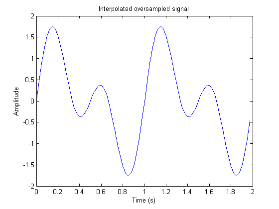
%Figure 2 plots just our interpolated signal, but this time with lines connecting each point.
figure(2)
plot(t1, x1, 'b-');
title('Interpolated oversampled signal');
xlabel('Time (s)');
ylabel('Amplitude');

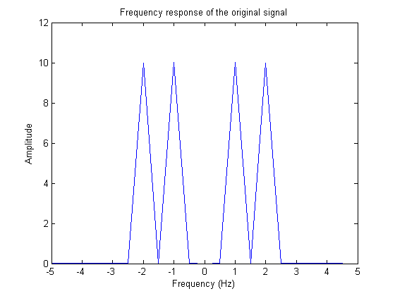
%Figure 3 plots the frequency response of our original sampled signal.
figure(3)
f = -1/(2*T):1/(N*T):1/(2*T)-1/(N*T);
plot(f,abs(fftshift(X)))
title('Frequency response of the origianl signal');
xlabel('Frequency (Hz)');
ylabel('Amplitude');
To run this script, you'll also need another script, called "u.m" with the following contained inside. This must be located in the same folder as the main script above.
function [out] = u(t)
out=(1+sign(t))./2;
end
I couldn't find MATLAB's step function, so I created my own.
Graphs

