Laplace transforms:Mass-Spring Oscillator

Problem Statement

Part 1

An ideal mass m=10kg is sitting on a plane, attached to a rigid surface via a spring. The spring with k=500N/m is exerting zero force when the mass is centered at x=0. Between the mass and plane there is a 1 mm layer of a viscous fluid and the block has an area of .1m^2 in contact the plane. Find the equation of motion that the spring mass system follows if there is an initial impulse applied, and then find the viscosity value of the fluid so that the mass comes to a stop within three seconds with the initial impulse used. Below is a picture/FBR of the system.

Fig. 1

As set up, the mass is sitting at x=0 with positive being to the right.

Part 2

Apply the Initial Value and Final Value Theorems to this problem.

Part 3

Make a bode plot.

Part 4

Find how to use the break points and asymptotes to obtain the magnitude frequency response.

Part 5

Use convolution to find the output.

Solution

Part 1

Using the FBR from the problem statement we can set up our differential equation:

$m{\ddot {x}}+b{\dot {x}}+kx=\delta (t)$

${\ddot {x}}+{\frac {b}{m}}{\dot {x}}+{\frac {k}{m}}x={\frac {\delta (t)}{m}}$

We now have a second order differential equation that governs the motion of the mass. If we make our initial conditions equal to zero, we save a few steps. Taking the Laplace transform of both sides gives:

${\mathcal {L}}_{s}\left\{{\frac {\delta (t)}{m}}\right\}={\mathcal {L}}_{s}\left\{{\ddot {x}}+{\frac {b}{m}}{\dot {x}}+{\frac {k}{m}}x\right\}$

${\frac {1}{m}}{\mathcal {L}}_{s}\left\{\delta (t)\right\}={\mathcal {L}}_{s}\left\{{\ddot {x}}\right\}+{\frac {b}{m}}{\mathcal {L}}_{s}\left\{{\dot {x}}\right\}+{\frac {k}{m}}{\mathcal {L}}_{s}\left\{x\right\}$

${\frac {1}{m}}\left\{1\right\}=\mathbf {X} (s)s^{2}+{\frac {b}{m}}\mathbf {X} (s)s+{\frac {k}{m}}\mathbf {X} (s)$

${\frac {1}{m}}=\left\{s^{2}+{\frac {b}{m}}s+{\frac {k}{m}}\right\}\mathbf {X} (s)$

Now that we have the Laplace transform of the differential equation that governs the motion of the spring and mass system, we need to solve for X(s):

$\mathbf {X} (s)={\frac {\frac {1}{m}}{\left\{s^{2}+{\frac {b}{m}}s+{\frac {k}{m}}\right\}}}$

We now have the function in terms of X(s). We will use the above equation to help in part 3, but for now we want to continue with part 1. We now want to find the value of b so that the mass stops oscillating after t=3s. However, we know that it will never actually be zero until a long time after, so for now we will consider motion >2% of original to be stopped. The below formula helps us find the value of b:

$t_{s}={\frac {4.6}{\zeta w_{n}}}$

${\frac {k}{m}}=w_{n}^{2}=50$

$\zeta ={\frac {4.6}{(3)(7.07)}}=0.2168$

Now using the relationship below, we are able to compute the value of b:

${\frac {b}{m}}=2\zeta w_{n}$

$b=\left\{(2)(0.2168)(7.07)(10)\right\}=30.667$

When we plug this number into the Laplace transform equation along with the values given:

$\mathbf {X} (s)={\frac {\frac {1}{10}}{\left\{s^{2}+{\frac {30.667}{10}}s+{\frac {500}{10}}\right\}}}$

$\mathbf {X} (s)={\frac {0.1}{\left\{s^{2}+3.066s+50\right\}}}$

The next step of taking the inverse Laplace transform is pretty complicated since we have complex roots, so I will just show the equation after it has been put back through:

$x(t)=0.2cos(6.9029t)e^{-1.533t}\,$

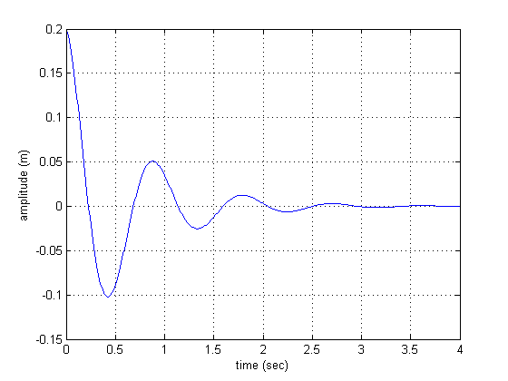
If we want to plot the equation above to see whether or not it looks good, we can use the below code in Matlab:

t=0:.01:4;
x=0.2.*cos(6.9029.*t).*exp(-1.533.*t);
plot(t,x);
grid
xlabel('time (sec)');
ylabel('amplitude (m)');

Fig. 1

Well, it looks good within that 2% value that we were looking for.

We have found the equation that the mass follows with the value of b that brings the mass to a "stop" within three seconds. But now we need to find the viscosity of the fluid that goes with that b value.

The equation below is one of the standard shear stress equations:

$\tau =\mu {\frac {\dot {x}}{t}}$.....where $t$ is the film thickness and $\mu$ is the kinematic viscosity.

We know that force is just a certain stress applied to an area, so:

$b{\dot {x}}=\mu A{\frac {\dot {x}}{t}}$

$b=\mu {\frac {A}{t}}$

Now we just plug in the values that are given and what we have found and we get:

$30.667=\mu {\frac {.1}{.001}}$

$\mu =0.3067{\frac {kg}{ms}}$

We have now found the viscosity value of the fluid used to damper the system. If we look that value up in a book, we find that this is about the viscosity of some SAE-10W oils at reasonable temperatures.

Part 2

The Initial Value Theorem states:

$\lim _{s\to \infty }s\mathbf {X} (s)=x(o)$

So if we plug our equation into this we have:

$\lim _{s\to \infty }s\left\{{\frac {0.1}{\left\{s^{2}+3.066s+50\right\}}}\right\}=x(o)$

$\lim _{s\to \infty }\left\{{\frac {0.1s}{\left\{s^{2}+3.066s+50\right\}}}\right\}=x(o)$

$\left\{0\right\}=x(o)$

As expected, the Initial Value Theorem shows us that the initial value is just the initial x value.

The Final Value Theorem States:

$x(\infty )=\lim _{s\to 0}s\mathbf {X} (s)$

$x(\infty )=\lim _{s\to 0}s\left\{{\frac {0.1}{\left\{s^{2}+3.066s+50\right\}}}\right\}$

$x(\infty )=\lim _{s\to 0}\left\{{\frac {0.1s}{\left\{s^{2}+3.066s+50\right\}}}\right\}$

$s\infty )=\left\{0\right\}$

As expected, the final value will be zero because the mass will come back to rest in the position from which it began at x=0.

Part 3

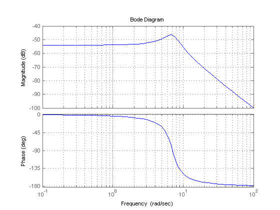
I used maple to plot the bode plots of the system using the below code which is pretty simple.

g = tf([.1],[1 3.066 50]);
bode(g);
grid 

Fig. 2

Part 4

From the transfer function in the Laplace Transform section,

$H(s)={\frac {.1}{s^{2}+3.066s+50}}$

it can be seen that there are no zeros (no s variables in the numerator that would make the function equal zero), but there are places in the s-domain in the denominator that would exhibit some interesting behavior. This will occur when the $s^{2}$ and the $k/m$ term, in this case "50", are on the same order of magnitude. When this happens, one value will quit dominating the other, and therefore cause problems on the real-imaginary coordinate system. This point can be visually observed by finding the intersection of the asymptotes in the Bode Plot. Where they intersect is (roughly) a breakpoint. It looks as though this is also the max of the Bode Plot and possibly the resonant frequency.

Part 5

The convolution is a equation that relates the output to the input in terms of the transfer function. As derived in class, it is

$x(t)=x_{in}(t)*h(t)=\int _{0}^{t}{x(t_{0})\,h(t-t_{0})\,dt_{0}}$

Where $h(t)$ is the inverse laplace of the transfer function.

$h(t)={\mathcal {L}}^{-1}\left\{{\frac {.1}{s^{2}+3.066s+50}}\right\}=x(t)=0.2cos(6.9029t)e^{-1.533t}$

So

$x(t)=x_{in}(t)*h(t)=\int _{0}^{t}{\delta (t)0.2cos(6.9029(t-t_{0}))e^{-1.533(t-t_{0})}\,dt_{0}}$

To solve the integral, one must do two integration by parts, or alternatively plug it into a calculator, which yields

$x(t)={\frac {-3}{2120}}\,g\,\sin {\theta }\,e^{{\frac {-1}{6}}t}\left(159\cos {\left({\frac {{\sqrt {159}}\,t}{6}}\right)}+{\sqrt {159}}\sin {\left({\frac {{\sqrt {159}}\,t}{6}}\right)}-159\,e^{{\frac {1}{6}}t}\right)$

---

Written by: David Steinweg

Checked by: Nathan Reeves