Coupled Oscillator: horizontal Mass-Spring

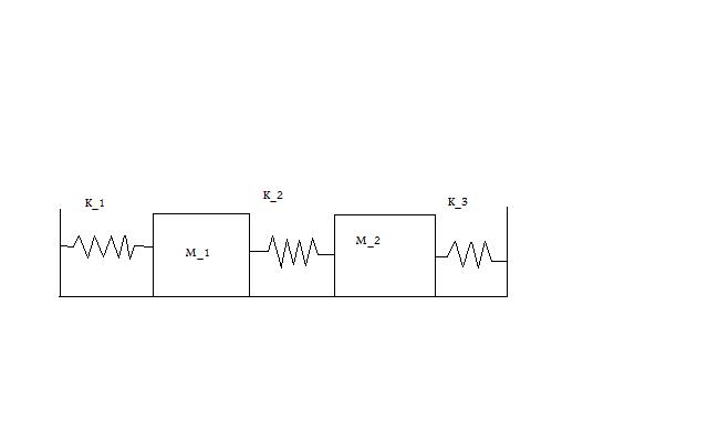
Problem Statement

Write up on the Wiki a solution of a coupled oscillator problem like the coupled pendulum. Use State Space methods. Describe the eigenmodes and eigenvectors of the system.

Initial Conditions:

$m_1=10kg$

$m_2=10kg$

$k1=25N/m$

$k2=75N/m$

$k3=50N/m$

Equations for M_1

$\begin{array}{rl}F& =ma\\ F& =m\ddot{x}\\ -k_1{x}_1-k_2(x_1{x}_2)& =m_1\ddot{x_1}\\ -\frac{k_1{x}_1}{m_1}-\frac{k_2(x_1-x_2)}{m_1}& =m_1\ddot{x_1}\\ -\frac{k_1{x}_1}{m_1}-\frac{k_2(x_1-x_2)}{m_1}& =\ddot{x_1}\\ -\frac{k_1+k_2}{m_1}{x}_1+\frac{k_2}{m_1}{x}_2& =\ddot{x_1}\\ \end{array}$

Equations for M_2

$\begin{array}{rl}F& =ma\\ F& =m\ddot{x}\\ -k_2(x_2-x_1)& =m_2\ddot{x_2}\\ \frac{-k_2(x_2-x_1)}{m_2}& =\ddot{x_2}\\ -\frac{k_2}{m_2}{x}_2+\frac{k_2}{m_2}{x}_1& =\ddot{x_2}\\ \end{array}$

Additional Equations

$\dot{x_1}=\dot{x_1}$

$\dot{x_2}=\dot{x_2}$

State Equations

$\left[\begin{array}{c}\dot{x_1}\\ \ddot{x_1}\\ \dot{x_2}\\ \ddot{x_2}\end{array}\right]$ = $\left[\begin{array}{cccc}0& 1& 0& 0\\ \frac{(k_1-k_2)}{m_1}& 0& \frac{-k_1}{m_1}& 0\\ 0& 0& 0& 1\\ \frac{k_1}{m_2}& 0& \frac{(k_1+k_2)}{m_2}& 0\end{array}\right]\left[\begin{array}{c}{x}_1\\ {\dot{x}}_1\\ x_2\\ {\dot{x}}_2\end{array}\right]+\left[\begin{array}{cccc}0& 0& 0& 0\\ 0& 0& 0& 0\\ 0& 0& 0& 0\\ 0& 0& 0& 0\end{array}\right]\left[\begin{array}{c}0\\ 0\\ 0\\ 0\end{array}\right]$

With the numbers...

$\left[\begin{array}{c}\dot{x_1}\\ \ddot{x_1}\\ \dot{x_2}\\ \ddot{x_2}\end{array}\right]$ = $\left[\begin{array}{cccc}0& 1& 0& 0\\ \frac{(-50N/m)}{10kg}& 0& \frac{-25N/m}{10kg}& 0\\ 0& 0& 0& 1\\ \frac{25N/m}{10kg}& 0& \frac{(100N/m)}{10kg}& 0\end{array}\right]\left[\begin{array}{c}{x}_1\\ {\dot{x}}_1\\ x_2\\ {\dot{x}}_2\end{array}\right]$

Eigen Values

Once you have your equations of equilibrium in matrix form you can plug them into MATLAB which will give you the eigen values automatically.

Given

$m_1=10kg$

$m_2=10kg$

$k_1=25\frac{N}{m}$

$k_2=50\frac{N}{m}$

We now have

$\left[\begin{array}{c}\dot{x_1}\\ \ddot{x_1}\\ \dot{x_2}\\ \ddot{x_2}\end{array}\right]=\left[\begin{array}{cccc}0& 1& 0& 0\\ -5& 0& -2.5& 0\\ 0& 0& 0& 1\\ 2.5& 0& 10& 0\end{array}\right]\left[\begin{array}{c}{x}_1\\ \dot{x_1}\\ x_2\\ \dot{x_2}\end{array}\right]+\left[\begin{array}{c}0\\ 0\\ 0\\ 0\end{array}\right]$

From this we get

${\lambda }_1=-3.0937,$

${\lambda }_2=2.1380i,$

${\lambda }_3=-2.1380i,$

${\lambda }_4=3.0937,$

Eigen Vectors

Using the equation above and the same given conditions we can plug everything into MATLAB and get the eigen vectors which we will denote as $k_1,k_2,k_3,k_4$.

$k_1=\left[\begin{array}{c}0.0520\\ -0.1609\\ -0.3031\\ 0.9378\end{array}\right]$

$k_2=\left[\begin{array}{c}0.4176i\\ -0.8928\\ -0.0716i\\ 0.1532\end{array}\right]$

$k_3=\left[\begin{array}{c}-0.4176i\\ -0.8928\\ 0.0716i\\ 0.1532\end{array}\right]$

$k_4=\left[\begin{array}{c}-0.0520\\ -0.1609\\ 0.3031\\ 0.9378\end{array}\right]$

So then the answer is...

We can now plug these eigen vectors and eigen values into the standard equation

$x=c_1{k}_1{e}^{{\lambda }_{1}t}+c_2{k}_2{e}^{{\lambda }_{2}t}+c_3{k}_3{e}^{{\lambda }_{3}t}+c_4{k}_4{e}^{{\lambda }_{4}t}$

$x=c_1$$\left[\begin{array}{c}0.0520\\ -0.1609\\ -0.3031\\ 0.9378\end{array}\right]$$e^{-3.0937}+c_2$$\left[\begin{array}{c}0.4176i\\ -0.8928\\ -0.0716i\\ 0.1532\end{array}\right]$$e^{2.1380i}+c_3$$\left[\begin{array}{c}-0.4176i\\ -0.8928\\ 0.0716i\\ 0.1532\end{array}\right]$$e^{-2.1380i}+c_4$$\left[\begin{array}{c}-0.0520\\ -0.1609\\ 0.3031\\ 0.9378\end{array}\right]$$e^{3.0937}$

Matrix Exponential

We now use matrix exponentials to solve the same problem.

$z=Tx$

So from the above equation we get this to prove the matrix exponetial works.

$\dot{z}=TA{T}^{-1}z$

We also know what T equals and we can solve it for our case

$T^{-1}=[k_1|k_2|k_3|k_4]$

$T^{-1}=\left[\begin{array}{cccc}0.0520& 0.4176i& -0.4176i& -0.0520\\ -0.1609& -0.8928& -0.8928& -0.1609\\ -0.3031& -0.0716i& 0.0716i& 0.3031\\ 0.9378& 0.1532& 0.1532& 0.9378\end{array}\right]$

Taking the inverse of this we can solve for T

$T=\left[\begin{array}{cccc}0& 0& 0& 0\\ 0& 0& 0& 0\\ 0& 0& 0& 0\\ 0& 0& 0& 0\end{array}\right]$

So taking

$\dot{z}=TA{T}^{-1}z$

We get the uncoupled matrix of

$\dot{z}=\left[\begin{array}{cccc}-3.0937& 0& 0& 0\\ 0& 2.1380i& 0& 0\\ 0& 0& -2.1380i& 0\\ 0& 0& 0& 3.0937\end{array}\right]$