Chris' Page for HW 13 (Sampling at 3Hz)

Sample $sin(2\pi nt)$ at 3 Hz; take the DFT, explain the results.

t1 = 0:1/3:3;
t2 = 0:1/1000:3;
y1 = sin(2*pi*t1);
y2 = sin(2*pi*t2);
NFFT1 = 2^nextpow2(length(y1));
NFFT2 = 2^nextpow2(length(y2));
Y1 = fft(y1,NFFT1)/length(y1);
Y2 = fft(y2,NFFT2)/length(y2);


f1 = 1/3./(2*linspace(0,1,NFFT1/2));
f2 = 10000./(2*linspace(0,1,NFFT2/2));

figure(2)
hold on
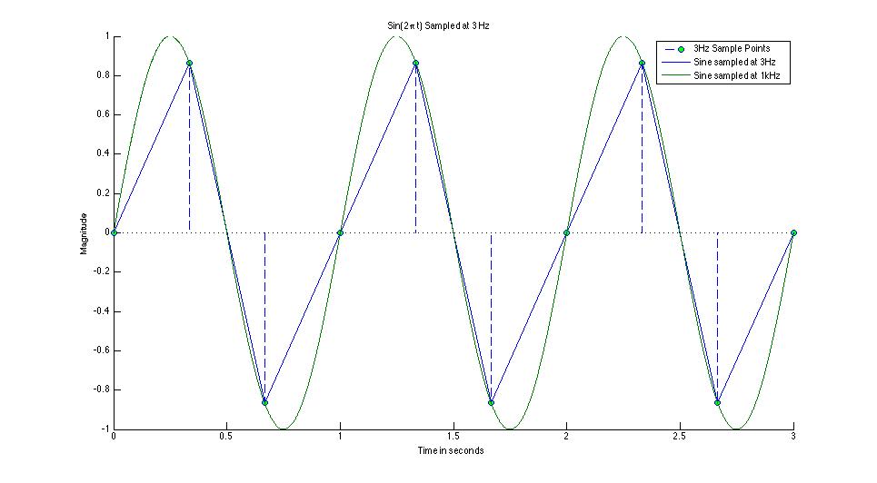
h = stem(t1(1:10),y1(1:10),'fill','--');
set(get(h,'BaseLine'),'LineStyle',':')
set(h,'MarkerFaceColor','green')
plot(t1(1:10),y1(1:10), t2(1:3000), y2(1:3000))
legend('3Hz Sample Points','Sine sampled at 3Hz','Sine sampled at 1kHz')
xlabel('Time in seconds')
ylabel('Magnitude')
title('Sin(2\pi t) Sampled at 3 Hz')
hold off

figure(3)
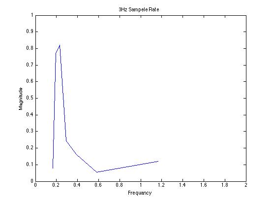
plot(f1,2*abs(Y1(1:NFFT1/2)))
axis([0 2 0 1])
title('3Hz Sampele Rate')
xlabel('Frequancy')
ylabel('Magnitude')

figure(4)
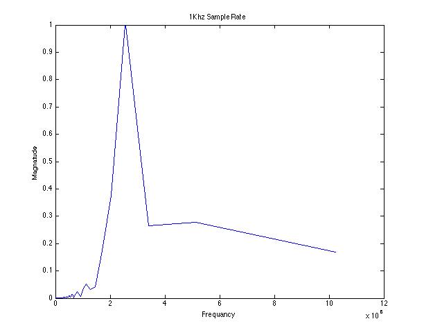
plot(f2,2*abs(Y2(1:NFFT2/2)))
axis([0 12000000 0 1])
title('1Khz Sample Rate')
xlabel('Frequancy')
ylabel('Magnatude')

---

With only 3 samples points per cycle the sinusoid looks like a triangle wave. Having too few sample points results in a DFT with edge effects that are large compared to the actual signal. As the number of sample points increases the accuracy of the digitized function increases and the DFT becomes a better representation of the true frequency components.