DFT example using MATLAB - HW11
Max Woesner
Homework #11 - DFT example using MATLAB
Problem Statement
Present an Octave (or MATLAB) example using the discrete Fourier transform (DFT).
Solution
I decided to demonstrate aliasing for my MATLAB example using the DFT.
Aliasing occurs when you don't sample a signal fast enough to be able to reconstruct it accurately after sampling. To avoid this problem, we must follow Nyquist's theorem, which states that we must sample at a rate at least twice the fastest frequency of the signal we are sampling.
First, let's look at aliasing. Consider the MATLAB script below.
clear all;
close all;
f = 2; % sine wave frequency
fs = 3; % sample frequency
tmax = 2; % go to 2 seconds
T = 1/fs;
t = 0:0.001:tmax;
x = sin(2*pi*f*t);
ts = 0:T:tmax;
xs = sin(2*pi*f*ts);
xa = sin(2*pi*(f-fs)*t);
figure(1)
plot(t,x)
xlabel('Time (s)')
ylabel('Signal')
title('Original Signal x(t)')
figure(2)
plot(t, x, '-b', ts, xs, 'go', t, xa, 'r')
legend('Original signal x(t)', 'Sample points', 'Reconstructed signal');
xlabel('Time (s)')
ylabel('Signal')
title('Orignial Signal with Aliasing')
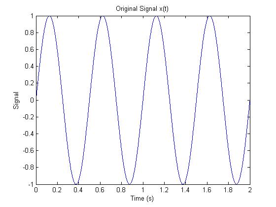
Here is the original signal to be sampled.
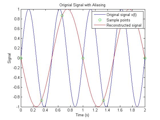
Here is the sampled signal added. Notice that the frequency is 1.5 times the highest frequency of the original signal, thus aliasing occurs, and the reconstructed signal is significantly different than the original signal.
Now let's consider the discrete Fourier transform of the original signal.
clear all;
close all;
f = 2; % sine wave frequency
tmax = 2; % go to 2 seconds
T = 0.01;
t = 0:T:tmax;
N = length(t);
x = sin(2*pi*f*t); % The original signal
X = fft(x); % The discrete Fourier transform
Xact = 0.*t; % The actual Fourier transform
Xact((N+1)/2-round(f*N*T)+1) = 0.5; % Simulates the delta function
Xact((N+1)/2+round(f*N*T)) = 0.5;
Xshft = fftshift(X); % To get the correct frequencies
f = -1/(2*T):1/(N*T):1/(2*T)-1/(N*T);
figure(1)
plot(t,x)
xlabel('Time (s)')
ylabel('Signal')
title('Original Signal x(t)')
figure(2)
plot(f, abs(X))
title('Unshifted Discrete Fourier Transform of x(t)')
xlabel('Frequency (s)')
ylabel('Magnitude of X(f)')
figure(3)
plot(f, abs(Xshft))
title('Shifted Discrete Fourier Transform of x(t)')
xlabel('Frequency (s)')
ylabel('Magnitude of X(f)')
figure(4)
plot(f, Xact)
title('Actual Fourier Transform of x(t)')
xlabel('Frequency (s)')
ylabel('Magnitude of X(f)')
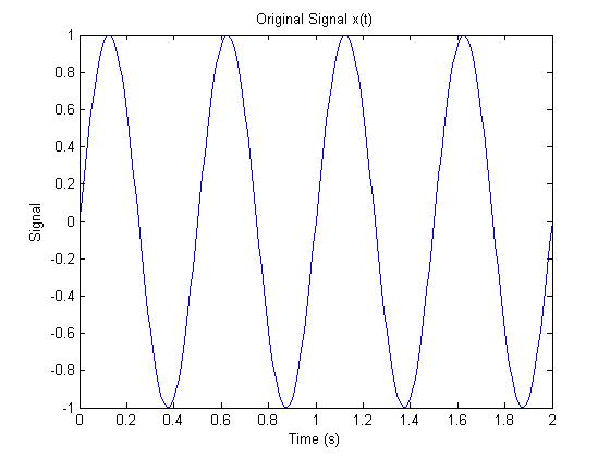
Here is the original signal again.
Using the fast Fourier transform (FFT) to obtain the discrete Fourier transform gives us this plot.
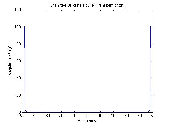
Since the FFT only shows the positive frequencies, we need to shift the graph to get the correct frequencies. The plot looks like this.
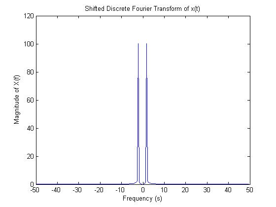
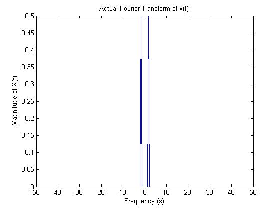
We can compare the DFT to the actual Fourier transform and see that they are very similar. The magnitude is different, and the DFT contains some extra frequencies from sampling.
