Fall 2009/JonathanS
Problem
A simple pendulum with a length L = 0.5m is pulled back and released from an initial angle . Then it is run with a forcing function of cos(3) Find an equation that gives the angle of the pendulum at any given time t.
Solution
Assuming no damping and a small angle(), the equation for the motion of a simple pendulum can be written as
Substituting values we get
Remember the identities
Now we can take the Laplace Transform to change the second order differential equation, from the t domain, into a simple linear equation, from the s domain, that's much easier to work with
Since we know that and the initial velocity we get
Now we can take the inverse Laplace Transform to convert our equation back into the time domain
This will give us the angle (in degrees) of the pendulum at any given time t.
Initial Value Theorem
We can use the Initial Value Theorem as a check that our initial values for the problem are valid.
Below we will use this theorem to check the values for our problem.
This value is the initial angle we gave the pendulum so it checks out.
Final Value Theorem
We can use the Final Value Theorem as a check that our final values for the problem are valid.
Below we will use this theorem to check the values for our problem.
This is zero because the average angle as time goes to infinity will be zero (halfway between -12 and 12 degrees).
Bode Plots
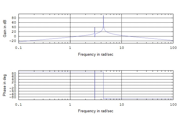
To find the bode plot we use the function
Entering this into a program such as Maple, Octave, or MATLAB will give you a plot that looks like this
Asymptotes & Break Points
In this section I will describe how you can use the transfer function to quickly estimate what the bode plot will look like.
To find the initial value we can take . Which gives us
From our original input we know that so
Now we can plug that into our log function
If we check that against our bode plot above we can see that this is pretty close. Now we can find the deflections using the transfer function. It will be easier to work with in factored form. For every "s" we have in the numerator we will increase the slope by 20db/decade. For every "s" we have in the denominator we will decrease the slope by 20db/decade. These changes will occur at the poles which form our break points and asymptotes.
We get asymptotes at s=3j and s=4.47j from the denominator. For our purposes we can just ignore the imaginary part. We should also have increases of 20db/decade at s=0 and s=3.01 which we find from the numerator.
Convolution
Convolution, by definition, states that H(s)=Y(s)/X(s) where H(s) is the transfer function, Y(s) is the output function, and X(s) is the input function. We would like to find the output of the system, so for our purposes we will rearrange the above equation like this.
State Space Equations
Now we can transfer the functions we already have into state space. This is simply taking our original differential equation and putting it in terms of vectors and matrices. This can make the equations easier to work with.
