Mark's Article on the DFT
Jump to navigation
Jump to search
The DFT
The Discrete Fourier Transform, or DFT for short, is the Fourier Transform in the discrete world. It is almost exactly like the Fourier Transform.
MATLAB script
clear all;
tmax = 1; %The signal will run from 0 to tmax (in seconds)
T=.01; %Sampling period
wf=5; %Waveform frequency: the frequency of the signal to transform
t=0:T:tmax;
N=length(t);
%x = sin(wf*pi*t)./(wf*pi*t); %This signal did not work out well
%x((N+1)/2) = 1;
x = sin(2*pi*wf*t); %This is the signal to transform
X = 0.*t; %The fourier transform of the signal x (calculated by hand)
X((N+1)/2-round(wf*N*T)+1) = 0.5; %I did this to simulate the delta function
X((N+1)/2+round(wf*N*T)) = 0.5;
Xdft = fftshift(x); %The DFT (Discrete Fourier Transform of the signal x)
Xdftu = fft(x); %The DFT (Discrete Fourier Transform of the signal x)
Xdft((N+1)/2:N) = Xdftu(1:(N+1)/2); %The fftshift didn't work for me
Xdft(1:(N+1)/2) = Xdftu((N+1)/2:N); %So this manually shifts the FFT
f = -1/(2*T):1/(N*T):1/(2*T)-1/(N*T);
figure(1)
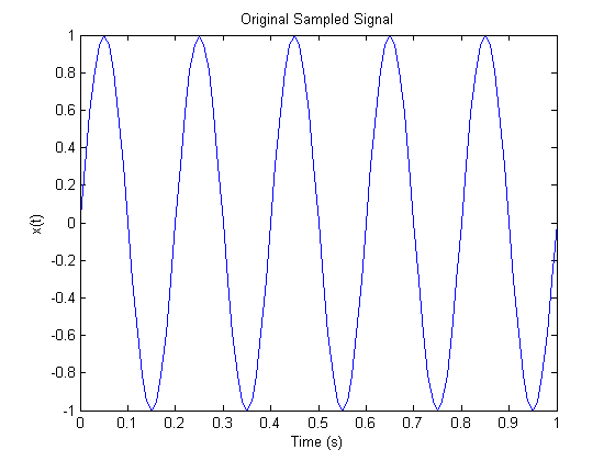
plot(t, x)
title('Original Sampled Signal')
xlabel('Time (s)')
ylabel('x(t)')
figure(2)
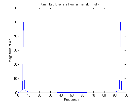
plot(f, abs(Xdftu))
title('Unshifted Discrete Fourier Transform of x(t)')
xlabel('Frequency')
ylabel('Magnitude of X(f)')
figure(3)
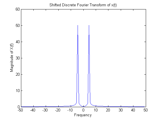
plot(f, abs(Xdft))
title('Shifted Discrete Fourier Transform of x(t)')
xlabel('Frequency')
ylabel('Magnitude of X(f)')
figure(4)
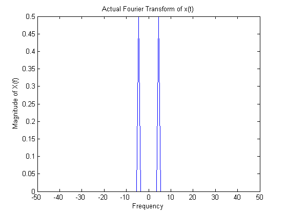
plot(f, X)
title('Actual Fourier Transform of x(t)')
xlabel('Frequency')
ylabel('Magnitude of X(f)')
Graphs


Explanations
I picked a sine wave of frequency 5 for my signal. (Shown in Figure 1.) I sampled it and took the discrete Fourier transform of the signal. (Shown in figure 2.) Using the FFT algorithm, the transform only shows the positive frequencies. You have to shift the graph to get the correct frequencies. Figure 3 shows the shifted (and now correct) graph. In Figure 4, I've shown the actual Fourier transform of the signal. As you can see, they are very similar. The heights are different and on the DFT graph, you'll see some frequencies other than the exact frequencies, but that is because of sampling.