CDPlayerJEW

How a CD Player Works

A CD player reads a dicrete set of data off a CD. In short, a CD player takes this data and sends it through a digitla to analog converter, then through a low pass filter, and finally is output through speakers. A simple diagram illustrates this below.

When an audio CD is recorded, the music has an infinite amount of data points and can be represented as a continuous function of time $x(t)$. Because a medium, such as a CD, has a finite amount of space, it will not be able to hold $x(t)$ since it has an infinite amount of data. Instead, the music is sampled at intervals to create a discrete function of time $x(nT)$ where $n$ is an integer and $T$ is the interval between samples.

This discrete signal can be represented mathematically by:

$\sum _{n=-\infty }^{\infty }x(nT)\delta (t-nT)$

Then, the discrete signal is convolved by the D/A converter with a function $p(t)$:

$p(t)=u\left(t+{\frac {T}{2}}\right)-u\left(t-{\frac {T}{2}}\right)$

$\sum _{n=-\infty }^{\infty }x(nT)\delta (t-nT)*p(t)=\sum _{n=-\infty }^{\infty }x(nT)p(t-nT)$

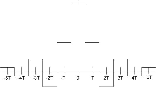
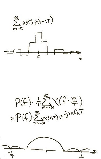
This convolution, which is the convolution of the discretized signal and $p(t)$, a pulse function, will yield a graph that is no longer discrete, but is stepped. The following is an example:

In the frequency domain, the above stepped signal will look like the following:

It turns out that the frequency graph shown above is very similar to the frequency graph of the original sound signal that was recorded. So, the signal is then sent to the speaker(s) for playback.

2x Oversampling

Some feel that the sound quality of the playback is increased through oversampling. Oversampling requires the signal processor to "fill in" the gaps in the discretized signal thus forming a smoother stepped graph. As noted above, the stepped graph is the result of convolving the discretized sound signal with a pulse function.

In order to perform oversampling, an extra step must be inserted into the process described above. The discretized time signal must be convolved with a function $h(t)$. The resulting convolution will then be convolved with the pulse function $p(t)$. This is the only change in the process.

$h(t)=\sum _{m=-M}^{M}h\left({\frac {mT}{n}}\right)\delta \left(t-{\frac {mT}{n}}\right)$

where $n$ is the number of times oversampling desired. In the case of 2x oversampling, $n=2$ and so,

$h(t)=\sum _{m=-M}^{M}h\left({\frac {mT}{2}}\right)\delta \left(t-{\frac {mT}{2}}\right)$

Graphically, this looks like this: File:2x01.jpgFile:2x02.jpg

Mathematically, the equation is:

$x(t)*h(t)=\sum _{n=-\infty }^{\infty }x(nT)\delta (t-nT)*\sum _{m=-M}^{M}h\left({\frac {mT}{2}}\right)\delta \left(t-{\frac {mT}{2}}\right)$ $={\hat {y}}(t)=\sum _{l=-\infty }^{\infty }\left(\sum _{m=-M}^{M}x\left({\frac {l-m}{2}}T\right)h\left({\frac {mT}{2}}\right)\right)\delta \left(t-{\frac {lT}{2}}\right)$

$h(t)$ effectively fills in the gaps by taking the average of two adjacent data points and placing a data point, whose value is the average of it's two adjacent points, half way in between.

This process can be extended to cover 4, 8, 16 or higher oversampling. The result is a smoother stepped function (in the time domain) and a frequency function that looks more and more like the original signal.

- Principle author of this page: Jeffrey Wonoprabowo

- Image of CD Player Diagram and Convolution by Aric Goe or Todd Caswell (not sure which since both of them had it on their pages)