HW11 Aliasing Example: Difference between revisions
No edit summary |
No edit summary |
||
| (4 intermediate revisions by the same user not shown) | |||
| Line 3: | Line 3: | ||
How often is often enough? Well, the Nyquist-Shannon sampling thereom says twice as much as the highest frequency. To be exact, the theorem states: "Exact reconstruction of a continuous-time baseband signal from its samples is possible if the signal is bandlimited and the sampling frequency is greater than twice the signal bandwidth." | How often is often enough? Well, the Nyquist-Shannon sampling thereom says twice as much as the highest frequency. To be exact, the theorem states: "Exact reconstruction of a continuous-time baseband signal from its samples is possible if the signal is bandlimited and the sampling frequency is greater than twice the signal bandwidth." | ||
So what happens when you sample as the Nyquist-Shannon thereom suggests | So what happens when you don't sample as the Nyquist-Shannon thereom suggests? I hate Matlab, but in the self-sacrificing spirit I have towards you, my dear reader, I will use everything in my power including Matlab to clarify things. | ||
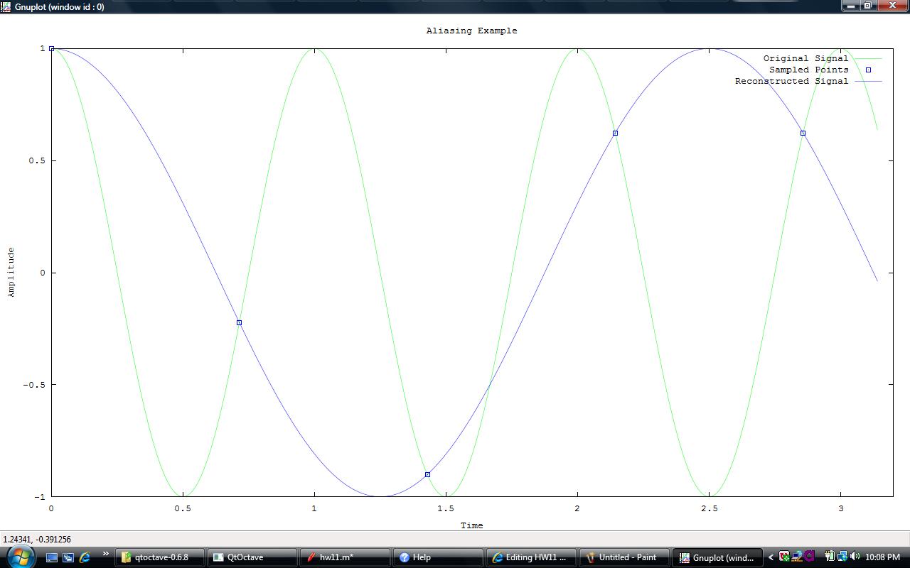
In the following picture, I have sampled the waveform at a rate higher than it's frequency, but less than twice the frequency. As you can see, the reconstructed signal is | |||
nowhere near the original signal. | |||
[[Image:sally1.jpg]] | |||
Octave Script: | |||
frequency = 1; | |||
sample = 1.4; | |||
T = 1/sample %period | |||
t = 0:0.01:3.14; %graph accuracy to .01 | |||
signal = cos(2*pi*t); %original signal | |||
ts = 0:T:3.14; | |||
sampledpoints = cos(2*pi*frequency*ts); | |||
reconstructed = cos(2*pi*(frequency-sample)*t); | |||
plot(t, signal, 'g', ts, sampledpoints, 'p',t, reconstructed, 'b') | |||
legend('Original Signal', 'Sampled Points', 'Reconstructed Signal') | |||
xlabel('Time') | |||
ylabel('Amplitude') | |||
title('Aliasing Example') | |||
So it has the same shape, but as you can see the frequency is alot lower than the original. Basically what not sampling enough does is that it recognizes multiple frequencies as the same frequency, so you lose crucial details in the reproduction of a sound. | So it has the same shape, but as you can see the frequency is alot lower than the original. Basically what not sampling enough does is that it recognizes multiple frequencies as the same frequency, so you lose crucial details in the reproduction of a sound. | ||
Latest revision as of 15:47, 3 December 2007
Aliasing - This is when you're sampling a function, but you don't sample often enough to reconstruct the waveform as it was before.
How often is often enough? Well, the Nyquist-Shannon sampling thereom says twice as much as the highest frequency. To be exact, the theorem states: "Exact reconstruction of a continuous-time baseband signal from its samples is possible if the signal is bandlimited and the sampling frequency is greater than twice the signal bandwidth."
So what happens when you don't sample as the Nyquist-Shannon thereom suggests? I hate Matlab, but in the self-sacrificing spirit I have towards you, my dear reader, I will use everything in my power including Matlab to clarify things.
In the following picture, I have sampled the waveform at a rate higher than it's frequency, but less than twice the frequency. As you can see, the reconstructed signal is nowhere near the original signal.
Octave Script:
frequency = 1;
sample = 1.4;
T = 1/sample %period
t = 0:0.01:3.14; %graph accuracy to .01
signal = cos(2*pi*t); %original signal
ts = 0:T:3.14;
sampledpoints = cos(2*pi*frequency*ts);
reconstructed = cos(2*pi*(frequency-sample)*t);
plot(t, signal, 'g', ts, sampledpoints, 'p',t, reconstructed, 'b')
legend('Original Signal', 'Sampled Points', 'Reconstructed Signal')
xlabel('Time')
ylabel('Amplitude')
title('Aliasing Example')
So it has the same shape, but as you can see the frequency is alot lower than the original. Basically what not sampling enough does is that it recognizes multiple frequencies as the same frequency, so you lose crucial details in the reproduction of a sound.
