Derivative Matrix for a Function Vector: Difference between revisions
John.hawkins (talk | contribs) Main Content |
John.hawkins (talk | contribs) Moving code to its own page |
||
| (2 intermediate revisions by the same user not shown) | |||
| Line 41: | Line 41: | ||
</math></center> | </math></center> | ||
Note that we need to divide by <math>1/2(\Delta x)</math> because the distance between <math>x_{m-1}</math> and <math>x_{m+1}</math> is <math>2\Delta x</math>. Similarly, the nonzero entries in the first and last rows are 2 to cancel out the 2 in the denominator. | Note that we need to divide by <math>1/2(\Delta x)</math> because the distance between <math>x_{m-1}</math> and <math>x_{m+1}</math> is <math>2\Delta x</math>. Similarly, the nonzero entries in the first and last rows are 2 to cancel out the 2 in the denominator. Using this matrix, we find that | ||
<center><math> | |||
\left(\frac{d}{dx}\right)y=\dfrac{1}{2(\Delta x)}\begin{bmatrix} | |||
-2&2&0&0&&&&&\\ | |||
-1&0&1&0&&&\cdots&&\\ | |||
0&-1&0&1&&&&&\\ | |||
\\ | |||
&&&&\ddots&&&&\\ | |||
\\ | |||
&\vdots&&&&-1&0&1&0\\ | |||
&&&&&0&-1&0&1\\ | |||
&&&&&0&0&-2&2 | |||
\end{bmatrix} | |||
\begin{bmatrix}y(x_1)\\y(x_2)\\y(x_3)\\ \\ \vdots \\ \\ y(x_{n-2})\\y(x_{n-1})\\y(x_n)\end{bmatrix} | |||
= | |||
\begin{bmatrix} | |||
\left[y(x_2)-y(x_1)\right]/\Delta x\\ | |||
\left[y(x_3)-y(x_1)\right]/2(\Delta x)\\ | |||
\left[y(x_4)-y(x_2)\right]/2(\Delta x)\\ | |||
\\ | |||
\vdots \\ | |||
\\ | |||
\left[y(x_{n-1})-y(x_{n-3})\right]/2(\Delta x)\\ | |||
\left[y(x_n)-y(x_{n-2})\right]/2(\Delta x)\\ | |||
\left[y(x_n)-y(x_{n-1})\right]/\Delta x | |||
\end{bmatrix} | |||
</math></center> | |||
which corresponds with the slopes we wished to obtain. | |||
==Solution Picture== | |||
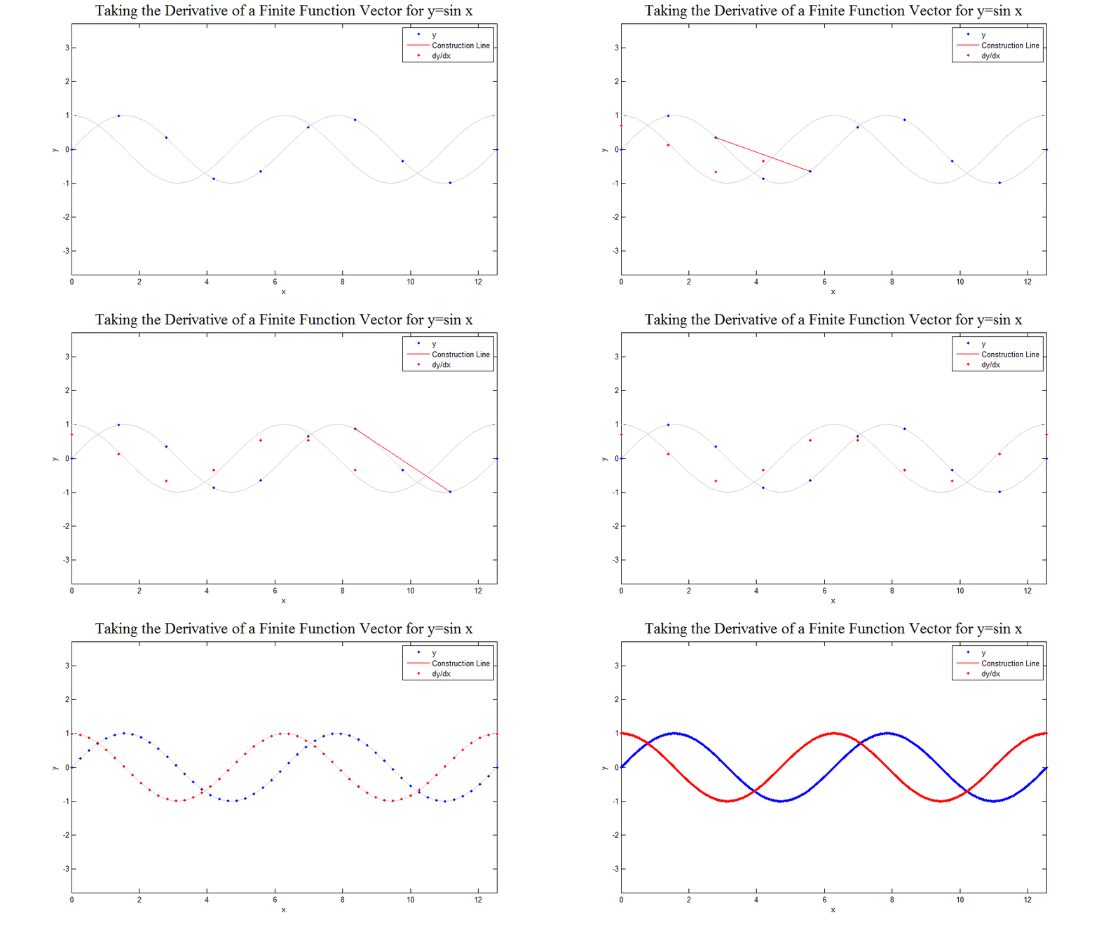
The figure below was created to demonstrate how the above matrix works. First, 10 points of the function are displayed. Then for each point the line between the two adjacent points is drawn and the slope of that line is shown to be <math>dy/dx</math> for the original point, calculated using the matrix shown above. After this has been done in the case of 10 points, the function and derivative vectors are shown for 15, 20, 30, 50, 100, 200, and 500 points. One can easily imagine the limiting case. The code used to develop this image can be found [[Derivative Operator Picture Code|here]]. | |||
[[Image:Derivative.gif]] | |||
==Reviewed By== | ==Reviewed By== | ||
Latest revision as of 23:18, 4 February 2010
Author
John Hawkins
Problem
The following problem statement is that proposed by Prof. Frohne on the main class page:
- Explore how a linear operator, like for example can be represented as some kind of a matrix multiply (with perhaps an infinite number of dimensions).
Solution
The solution presented here is limited to presenting a matrix representation of the operator .
First, let us consider the finite case. Let be the independent variable with components and let the components of be defined such that for all and for some constant . Also let . We wish to find the slope of the function at for any . To do this for the finite case, we will approximate the slope at a point as being the slope of the line between the two points and given that . For the case when or , we approximate as the slope the lines between and respectively. These approximations are accomplished by the following matrix:
Note that we need to divide by because the distance between and is . Similarly, the nonzero entries in the first and last rows are 2 to cancel out the 2 in the denominator. Using this matrix, we find that
which corresponds with the slopes we wished to obtain.
Solution Picture
The figure below was created to demonstrate how the above matrix works. First, 10 points of the function are displayed. Then for each point the line between the two adjacent points is drawn and the slope of that line is shown to be for the original point, calculated using the matrix shown above. After this has been done in the case of 10 points, the function and derivative vectors are shown for 15, 20, 30, 50, 100, 200, and 500 points. One can easily imagine the limiting case. The code used to develop this image can be found here.
